
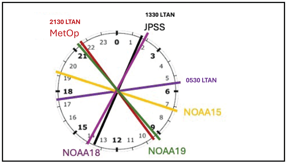
Figure 1
Local Time of Ascending Node (LTAN) of NOAA and EUMETSAT polar orbiting weather satellites as of July 24, 2024.
Table 1
Expected percentage of Earth observed by microwave sounders in a 24 hour cycle by two, three and six satellites in sun synchronous polar orbits, with each satellite at a different local time of ascending node (LTAN).
| REFRESH TIME (hr) | PERCENT OF EARTH COVERED | ||
|---|---|---|---|
| 2 PLATFORMS | 3 PLATFORMS | 6 PLATFORMS | |
| 0.5 | 10.91% | 16.84% | 30.35% |
| 1 | 20.64% | 31.53% | 53.75% |
| 2 | 39.87% | 55.94% | 81.60% |
| 3 | 52.69% | 74.78% | 94.43% |
| 4 | 64.73% | 90.06% | 98.75% |
| 6 | 81.92% | 97.02% | 99.63% |
| 8 | 94.03% | 98.59% | 99.84% |
| 12 | 99.22% | 99.64% | 100% |
| 24 | 100% | 100% | 100% |
| Orbital Planes | 2 | 3 | 6 |
| Orbit LTAN | 1330, 2130 | 0530, 1330, 2130 | 0530, 1330, 2130 |
| 0330, 0730, 1130 | |||
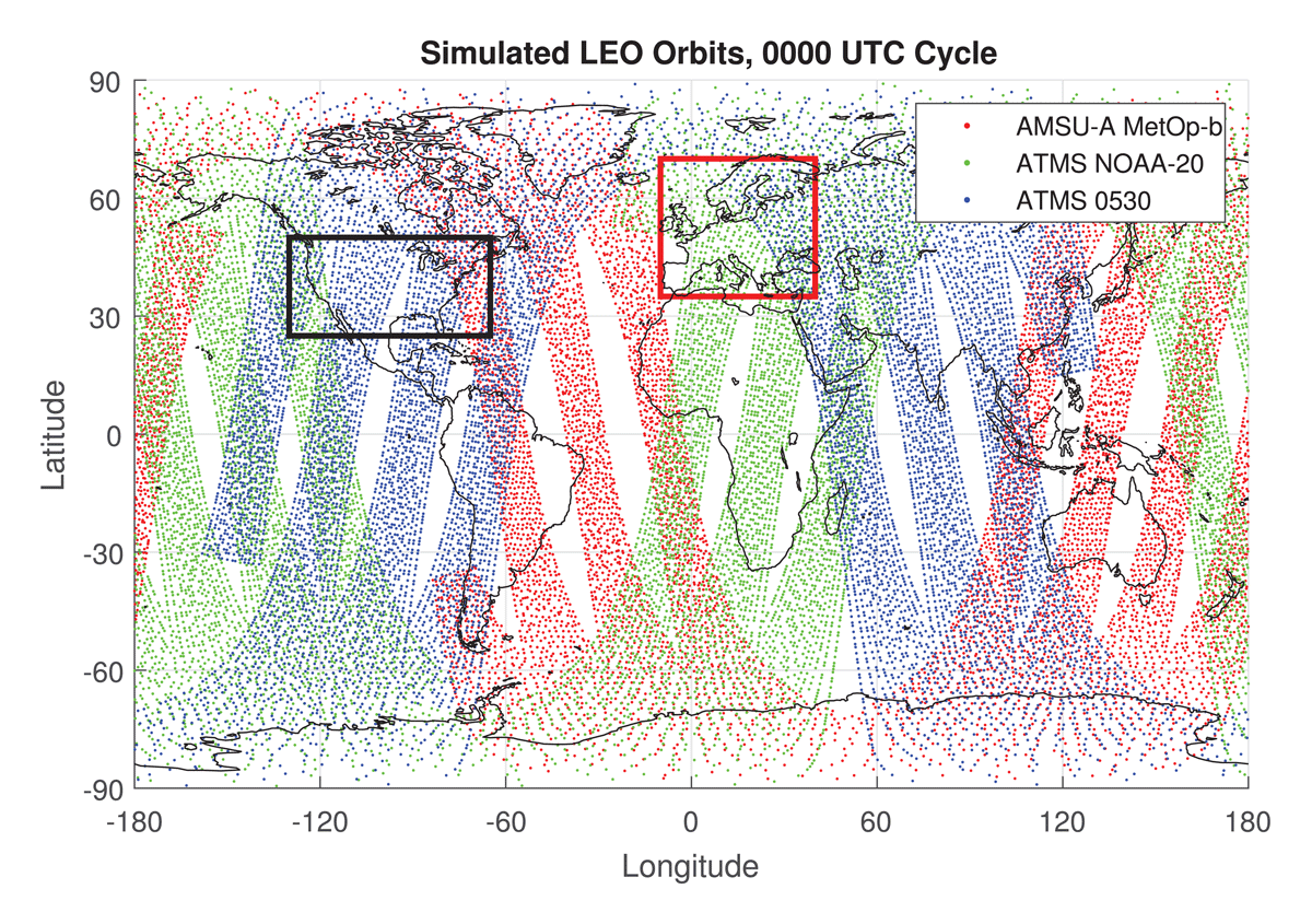
Figure 2
Simulated observation locations for July 1 0000 UTC cycle time (six-hour time window centered on 0000 UTC). Red, AMSU-A MetOp-b; green, ATMS NOAA-20; blue, ATMS 0530. Black box indicates the region used for CONUS calculations, red box indicates the region used for Europe calculations.
Table 2
Simulated observing platforms for the future global observing network experiments.
| INSTRUMENT | PLATFORM | FUTURE CONTROL | CrIS-ONLY | ATMS-ONLY | CrIS+ATMS |
|---|---|---|---|---|---|
| AMSR2 | GCOM W1 | X | X | X | X |
| AMSU-A | METOP-B | X | X | X | X |
| ATMS | NOAA-20 | X | X | X | X |
| ATMS | 0530 | X | X | ||
| CrIS-FSR | NOAA-20 | X | X | X | X |
| CrIS-FSR | 0530 | X | X | ||
| GEO IRS | GeoXO | X | X | X | X |
| GEO IRS | MTG | X | X | X | X |
| GEO IRS | Himawari | X | X | X | X |
| GMI | GPM | X | X | X | X |
| IASI | METOP-B | X | X | X | X |
| MHS | METOP-B | X | X | X | X |
| SSMIS | F17 | X | X | X | X |
| Surface conventional | X | X | X | X | |
| AMV | X | X | X | X | |
| Aircraft | X | X | X | X | |
| Scatterometer | X | X | X | X | |
| RAOB | X | X | X | X | |
| GNSS-RO | X | X | X | X |
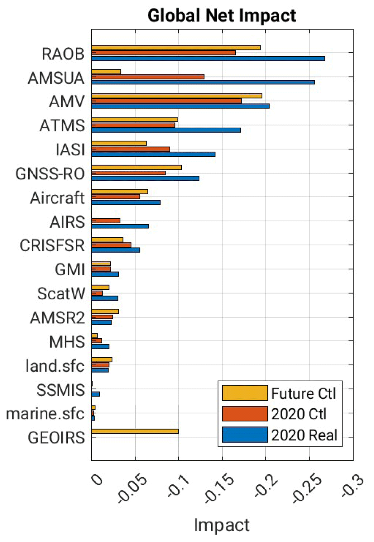
Figure 3
Comparison of FSOI estimates of observation impacts for the 2020 Control and Future Control in July compared to Real observations from 2020. 0000 UTC forecast cycle impacts on the 24-hour forecast of total wet energy error norm.
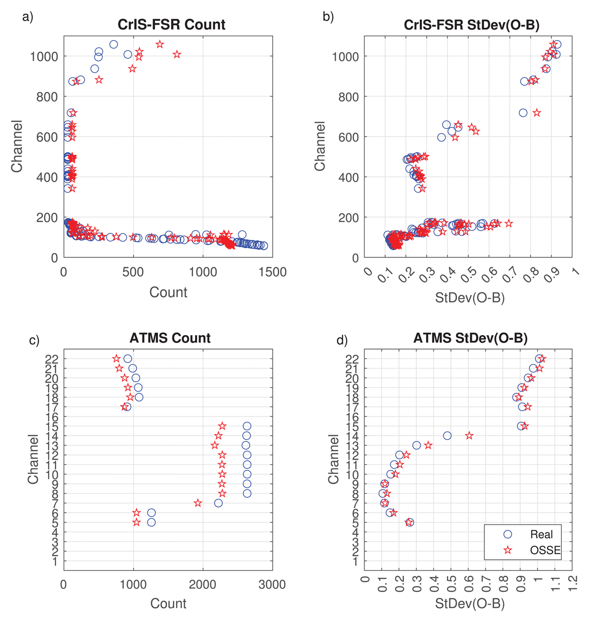
Figure 4
Calibration of simulated 0530 orbit CrIS-FSR and ATMS observations compared to real data. Blue circles, real data; red stars, simulated observations. One month of four times daily statistics of observation ingestion in the CrIS+ATMS case for July compared to the Real validation run using 2020 real data. a,b) CrIS-FSR NPP Real versus 0530 CrIS-FSR; c,d) Real ATMS NOAA-20 versus 0530 ATMS. a,c) Mean count of ingested observations per cycle time. b,d) Standard deviation of observation innovation (O-B).
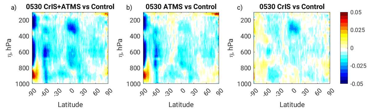
Figure 5
Fractional change to zonal mean temperature analysis RMSE compared to Future Control, July–Sept. Ordinate in model η level equivalent pressure. a) CrIS+ATMS case; b) ATMS-Only case; c) CrIS-Only case.
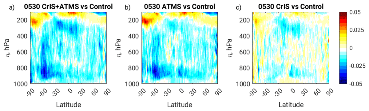
Figure 6
Fractional change to zonal mean specific humidity analysis RMSE compared to Future Control, July–Sept. Ordinate in model η level equivalent pressure. a) CrIS+ATMS case; b) ATMS-Only case; c) CrIS-Only case.
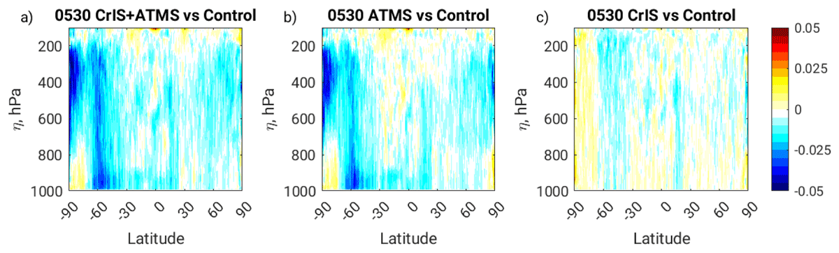
Figure 7
Fractional change to zonal mean zonal wind analysis RMSE compared to Future Control, July–Sept. Ordinate in model η level equivalent pressure. a) CrIS+ATMS case; b) ATMS-Only case; c) CrIS-Only case.
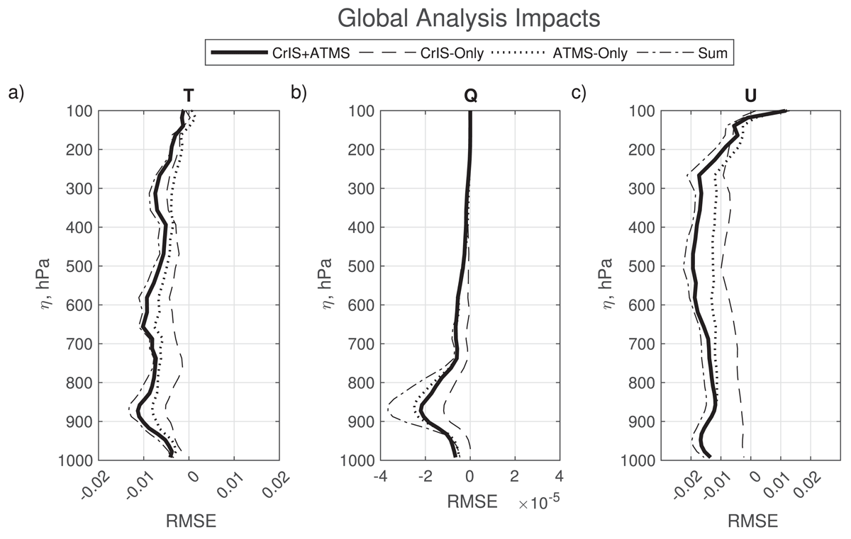
Figure 8
Difference in globally averaged temperature analysis RMSE compared to Future Control, July–Sept. Ordinate in model η level equivalent pressure. Heavy solid line, CrIS+ATMS; dashed line, CrIS-Only; dotted line, ATMS-Only; dot-dash line, sum of CrIS-Only and ATMS-Only. a) temperature, K; b) specific humidity, kgkg–1; c) zonal wind, ms–2.
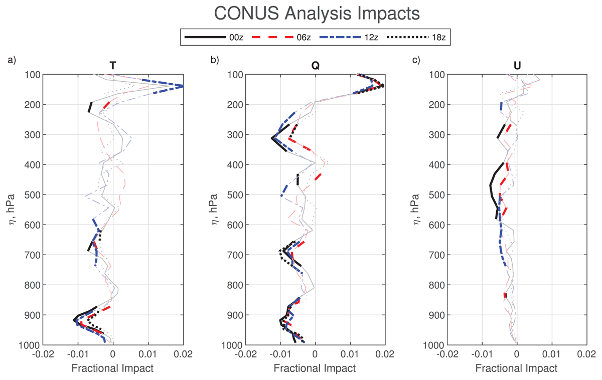
Figure 9
Fractional difference in globally averaged temperature analysis RMSE compared to Future Control over the CONUS region, July–Sept. Ordinate in model η level equivalent pressure. Heavy lines indicate significance at the 90% level. Solid black line, 0000 UTC cycle; dashed red line, 0600 UTC cycle, dash-dot blue line, 1200 UTC cycle; dotted black line, 1800 UTC cycle. a) temperature; b) specific humidity; c) zonal wind.
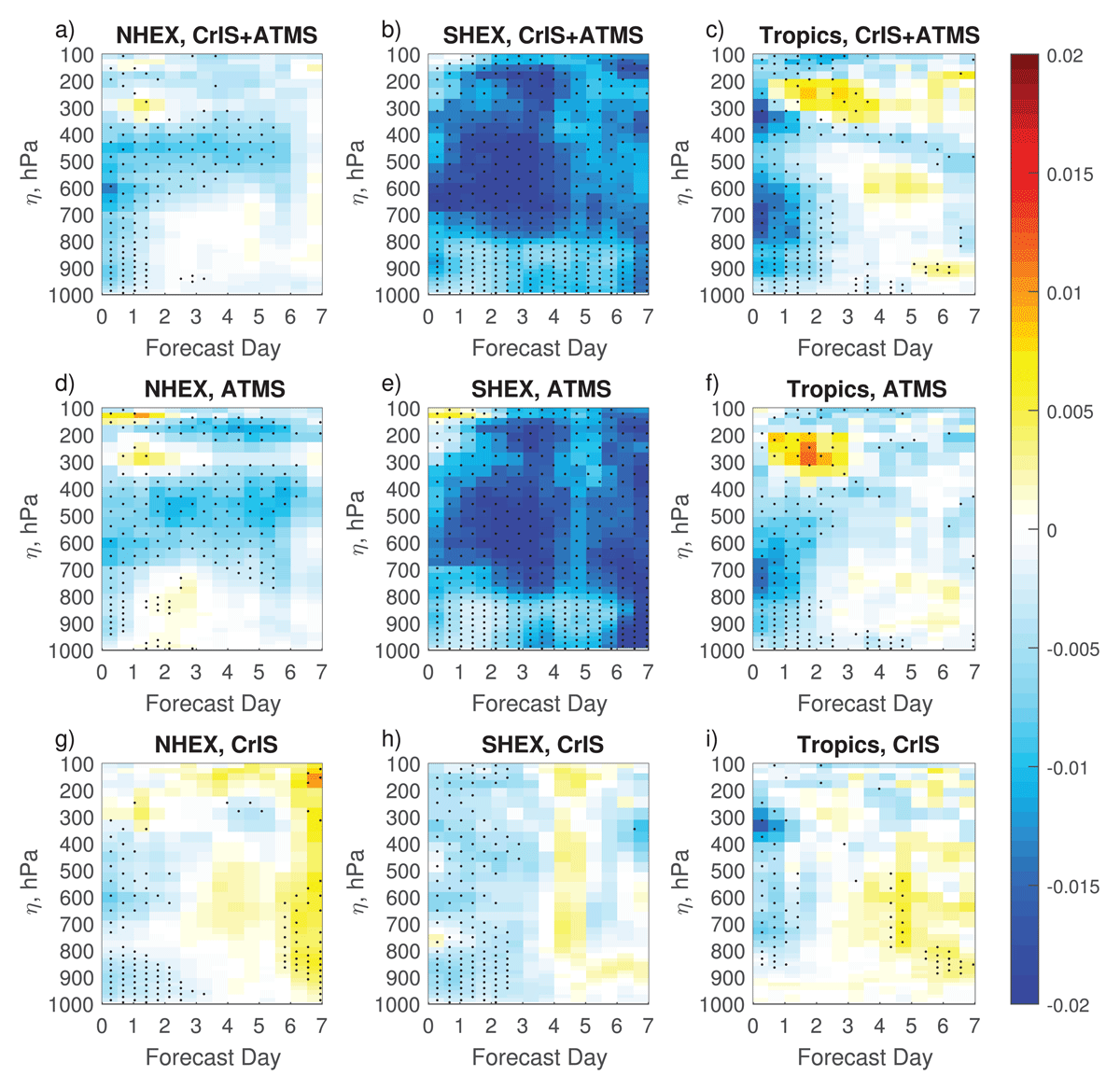
Figure 10
Fractional difference in regionally averaged temperature forecast RTMSE compared to and normalized by the Future Control RTMSE, July–Sept. Negative values indicate a reduction in forecast error compared to control. Stippling indicates 90% statistical significance. Ordinate in model η level equivalent pressure. a,b,c) CrIS+ATMS case; d,e,f) ATMS-Only case; g,h,i) CrIS-Only Case. a,d,g) NHEX region; b,e,h) SHEX region; c,f,i) Tropics region.
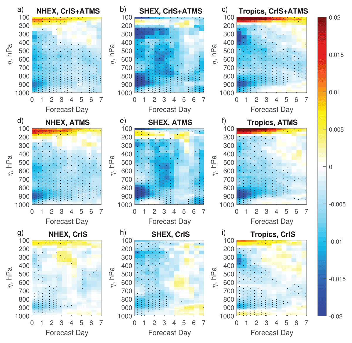
Figure 11
Fractional difference in regionally averaged specific humidity forecast RTMSE compared to and normalized by the Future Control RTMSE, July–Sept. Negative values indicate a reduction in forecast error compared to control. Stippling indicates 90% statistical significance. Ordinate in model η level equivalent pressure. a,b,c) CrIS+ATMS case; d,e,f) ATMS-Only case; g,h,i) CrIS-Only Case. a,d,g) NHEX regiona; b,e,h) SHEX region; c,f,i) Tropics region.
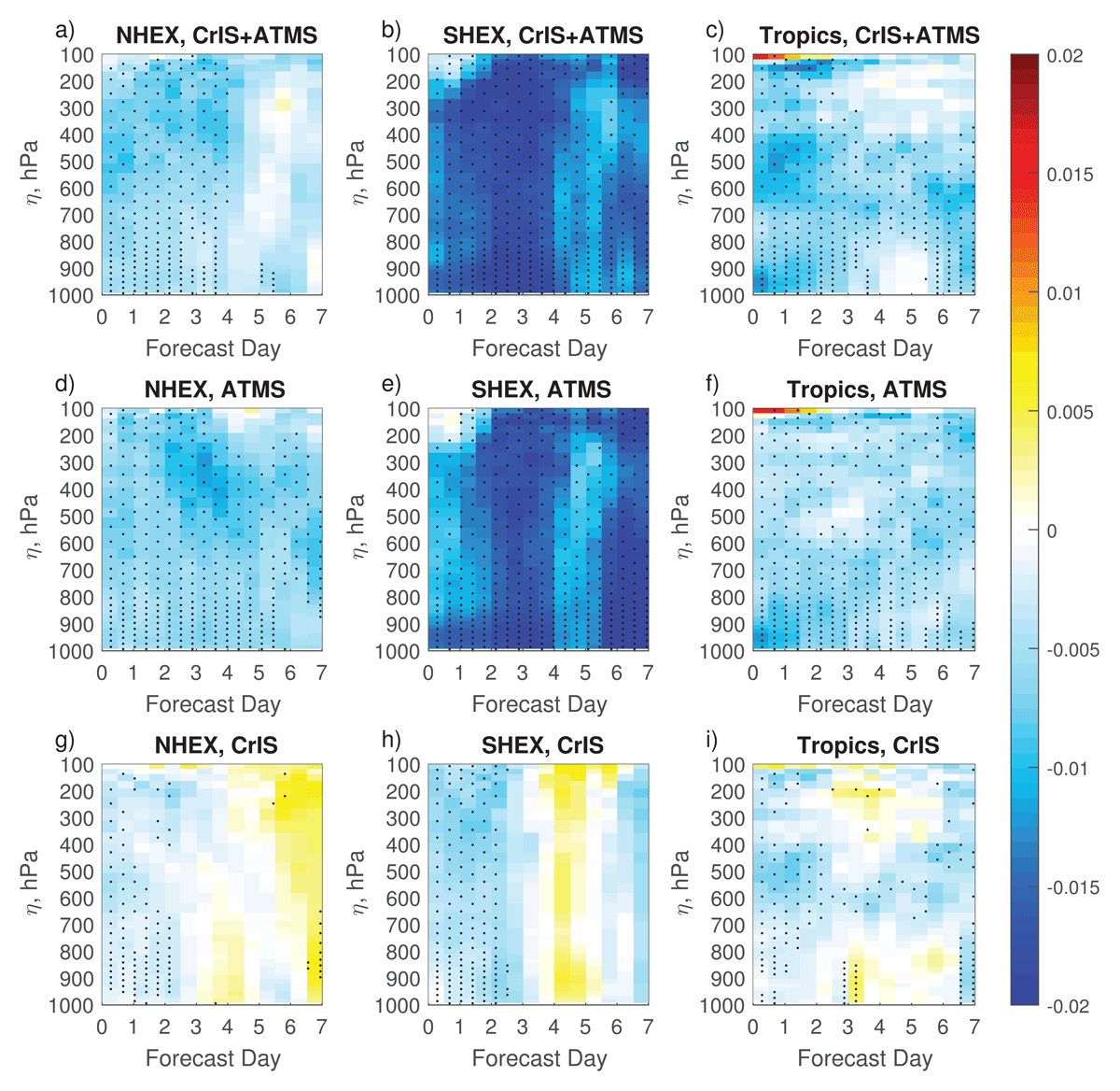
Figure 12
Fractional difference in regionally averaged zonal wind forecast RTMSE compared to and normalized by the Future Control RTMSE, July–Sept. Negative values indicate a reduction in forecast error compared to control. Ordinate in model η level equivalent pressure. Stippling indicates 90% statistical significance. a,b,c) CrIS+ATMS case; d,e,f) ATMS-Only case; g,h,i) CrIS-Only Case. a,d,g) NHEX region; b,e,h) SHEX region; c,f,i) Tropics region.
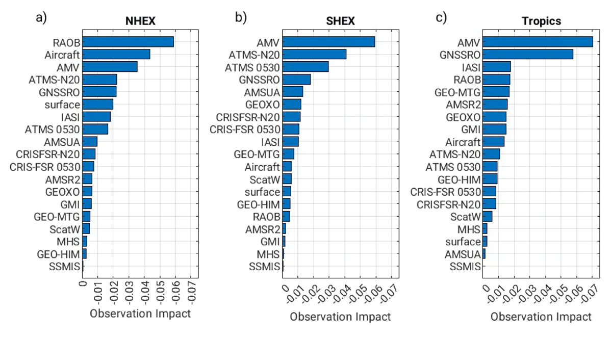
Figure 13
Four times daily forecast sensitivity observation impact for the CrIS+ATMS case using a 24-hour total wet energy error norm. July–September cycle mean net impact. Negative values indicate a reduction in forecast error, i.e. beneficial impact.
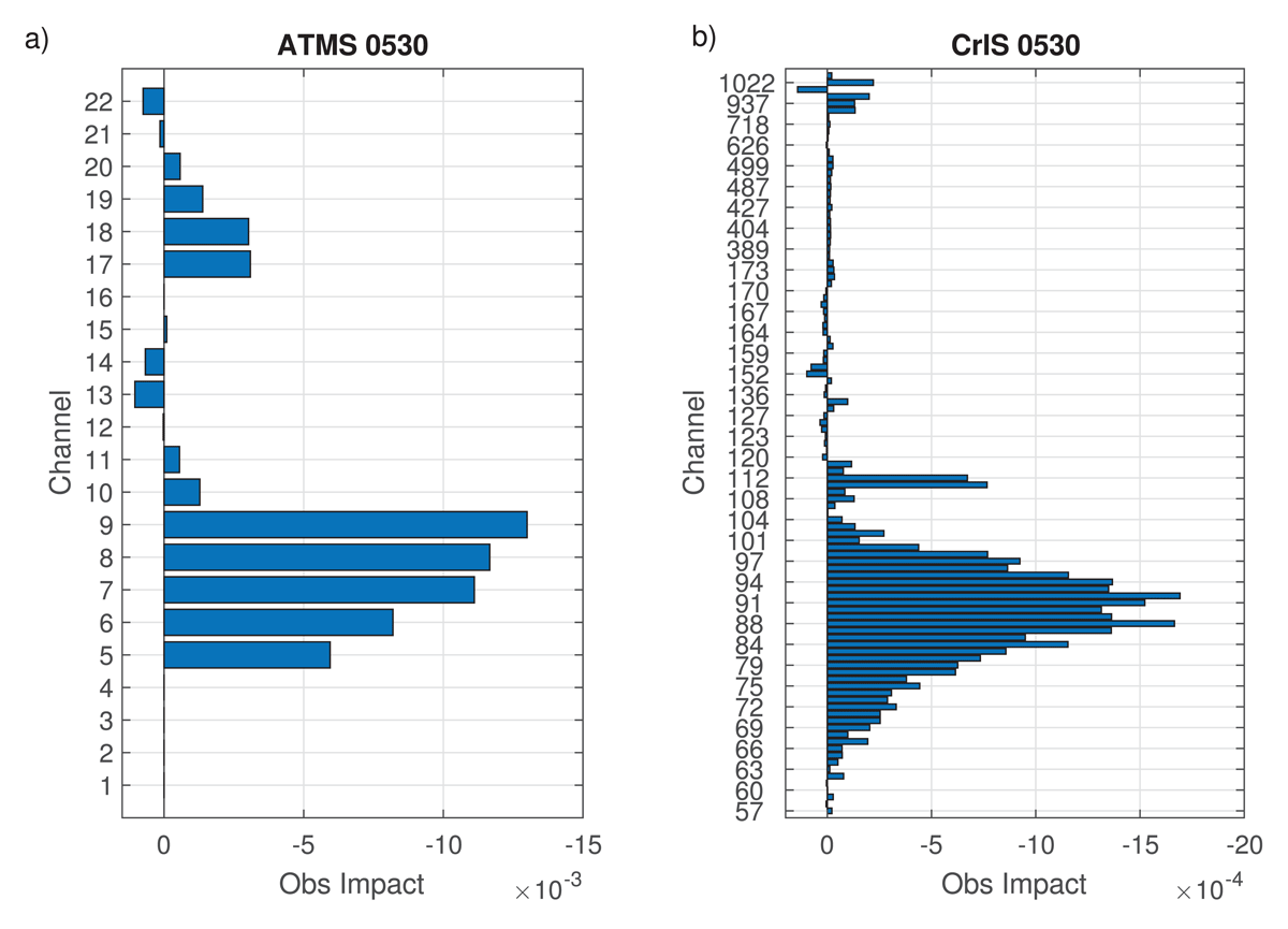
Figure 14
Four times daily forecast sensitivity observation impact per channel for the CrIS+ATMS case using a 24-hour total wet energy error norm. July–September cycle mean net impact. Negative values indicate a reduction in forecast error, i.e. beneficial impact. a) ATMS 0530 orbit; b) CrIS-FSR 0530 orbit.
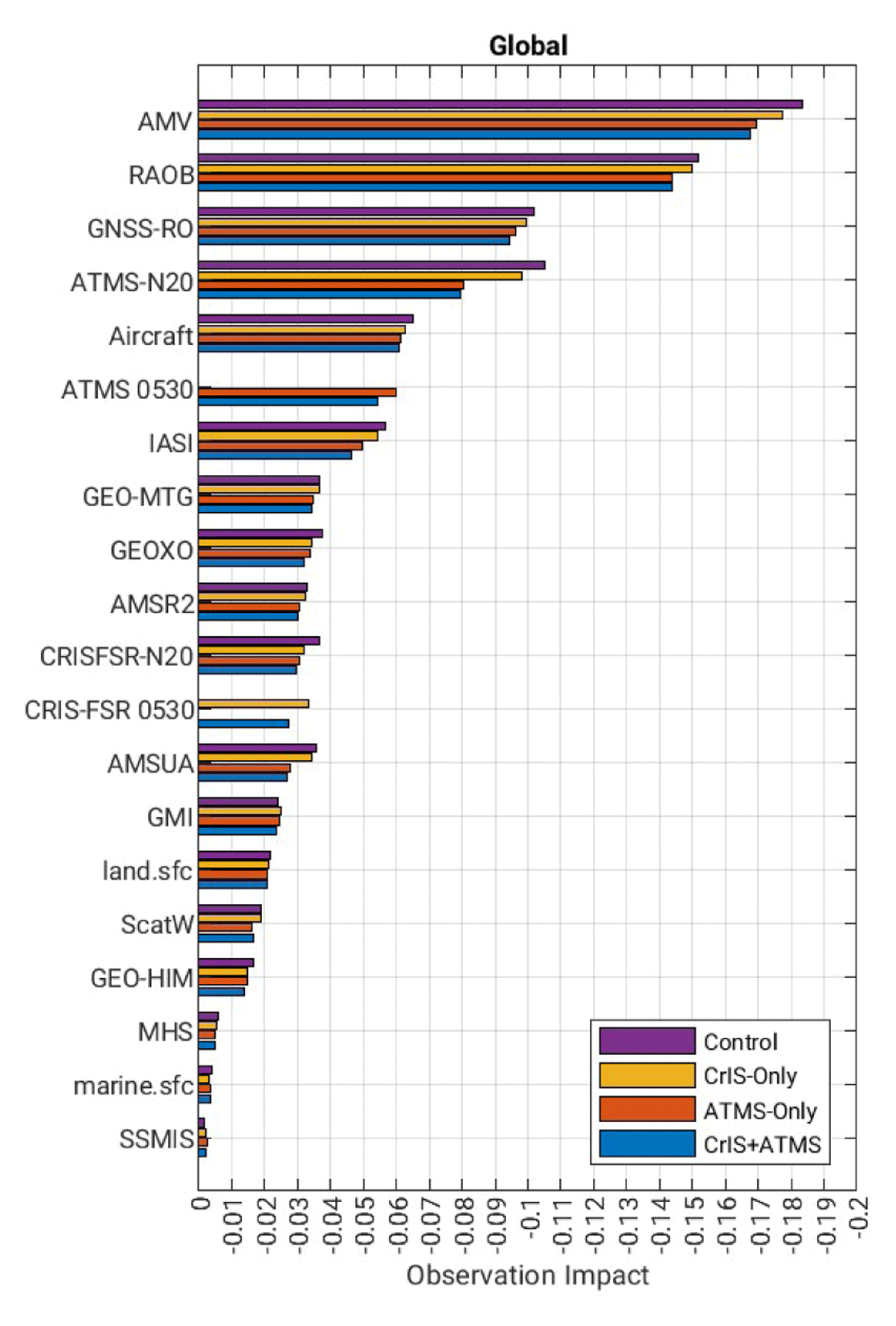
Figure 15
0000 UTC cycle forecast sensitivity observation impact using a 24-hour total wet energy error norm. July–September cycle mean net impact. Negative values indicate a reduction in forecast error, i.e. beneficial impact. Purple bars, Future Control case; yellow bars, CrIS-Only case; red bars, ATMS-Only case; blue bars, CrIS+ATMS case.
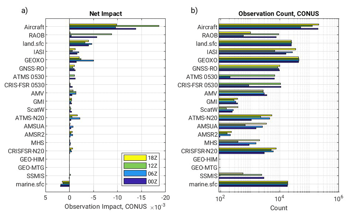
Figure 16
Comparison of forecast sensitivity observation impact over the CONUS region at different cycle times for the CrIS+ATMS case using a 24-hour total wet energy error norm. July–September cycle mean net impact. Negative values indicate a reduction in forecast error, i.e. beneficial impact. a) Net impacts; b) Observation counts (note semi-log).
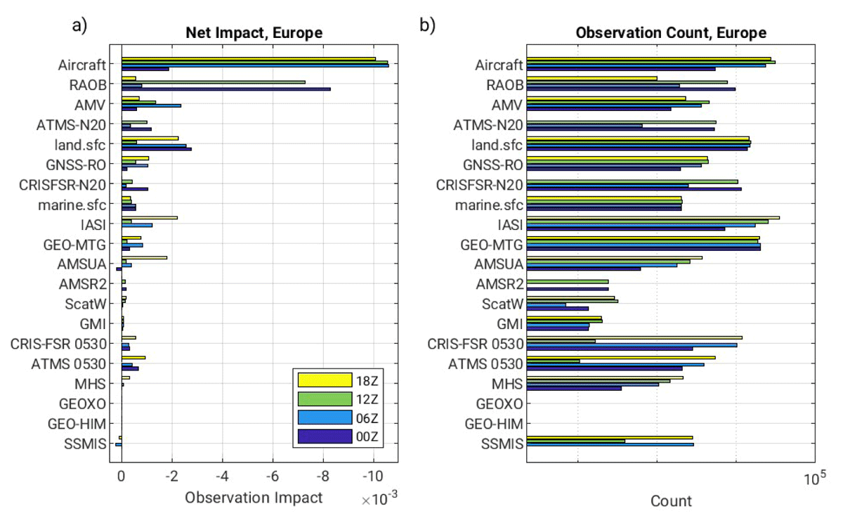
Figure 17
Comparison of forecast sensitivity observation impact over the Europe region at different cycle times for the CrIS+ATMS case using a 24-hour total wet energy error norm. July–September cycle mean net impact. Negative values indicate a reduction in forecast error, i.e. beneficial impact. a) Net impacts; b) Observation counts (note semi-log).
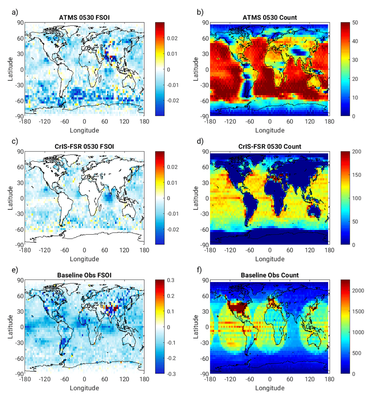
Figure 18
a,c,e) Sum of FSOI estimates of observation impact binned by location over the July–September period, 4 times daily FSOI data, CrIS+ATMS case. Negative values indicate a reduction in forecast error, i.e. beneficial impact. b,d,f) mean number of radiance observations ingested per cycle in bins of 4° latitude by 4° longitude. a,b) ATMS 0530 instrument; c,d) CrIS-FSR 0530 instrument; e,f) set of all conventional and remote sensed data types except for the 0530 platform.