
1 Introduction
According to modern concepts of dynamic meteorology, the mechanism of baroclinic instability is responsible for the genesis and development of synoptic-scale weather disturbances in the midlatitudes (Holton, 2004). This process is called cyclogenesis. In its basic features, this problem can be described within the framework of quasi-geostrophic theory, in which perturbations in the form of normal modes are superimposed on the basic state (most simply zonal flow). Under appropriate atmospheric conditions, perturbations can grow from their essentially infinitesimal amplitude into wave disturbances, and their subsequent transformation can give rise to synoptic-scale disturbances. From an energy point of view, this process represents a situation in which the available potential energy of the basic state is transferred to the energy of the perturbations, primarily to the available potential energy of the disturbances, which is further transformed into their kinetic energy. Baroclinic instability is related to the vertical gradient of wind velocity and through the thermal wind relation (see e.g., Holton, 2004; Bluestein, 1993) to the horizontal gradient of temperature.
The first studies of baroclinic instability were carried out independently by Charney (1947) and Eady (1949). Both authors worked with a vertically continuous model of the atmosphere and made several simplifications. In addition, Eady used simplifications in the atmosphere (e.g., f-plane) such that the problem could be solved analytically in an illustrative way.
In this paper, we derive explicit analytical relationships for wave-like perturbations in the fields of geopotential, temperature, isobaric divergence, and vertical velocity. In contrast to other analyses of the Eady model, we work with pressure as the vertical coordinate, i.e., in the p-system. This allows us to place the upper boundary condition at the upper boundary of the atmosphere for p approaching zero. Note that in the original Eady paper and later modifications (e.g., Haltiner and Williams, 1980; Holton, 2004; Pedlosky, 1987), the upper rigid boundary is placed at a finite height above the ground surface, which most often simulates the position of the tropopause. The use of the p-system allows us to naturally incorporate Earth’s surface topography.
In this article, we do not aim to provide a comprehensive overview of the various aspects of baroclinic instability. For this purpose, we refer to the existing monographs (e.g., Holton, 2004; Pedlosky, 1987; North et al., 2015; Grotjahn, 1993; Mak, 2011). The reader should also pay attention to the necessary condition for baroclinic instability by Charney and Stern (1962). Although Eady’s original work was published many years ago, the related topics are still actively researched, with recent relevant studies including Kalashnik and Chkhetiani (2018), Stamper and Taylor (2017) or Vic, Carton and Gula (2022).
2 Basic equations
The subject of our interest will be baroclinic instability on synoptic to planetary scales. The motions of such a scale can be described by the vorticity equation in the quasi-geostrophic approximation and by the thermodynamic equation in the adiabatic approximation:
where t is time, vψ = k × ∇pψ is the velocity vector of the non-divergent flow, ψ represents the stream function, and f0 is the value of the Coriolis parameter f at the reference mean latitude ϕ0, usually chosen as 45° N. It is clear from both Eqs. (1) and (2) we will continue to work in the p-system (standard coordinate system with p as vertical coordinate). Thus, ω has the meaning of the vertical velocity in the p-system, ω = dp/dt; ∇p is gradient in p-system; and σ represents parameter of static stability of the atmosphere (see Appendix for the definition). We refer the reader who is not familiar with the derivation of these equations to any of the following references: Holton (2004); Dutton (1986); Haltiner and Williams (1980). We remark that in the following we will assume a simplified geostrophic relationship between the geopotential ϕ and the stream function ϕ = f0ψ.
After some simple modifications, Eqs. (1) and (2) can be used to obtain
In the last equation, we can denote
We call the quantity Π the quasi-geostrophic potential vorticity and Eq. (3) is the quasi-geostrophic potential vorticity equation.
We assume that the state of the atmosphere can be decomposed into a basic state and at least an order of magnitude smaller perturbation. We will denote the basic state by a bar and the perturbation by a comma. Let the basic state be the purely zonal flow described by the geostrophic stream function , which corresponds to the velocity of zonal flow
The perturbation stream function is , . The resulting flow is then characterized by the stream function
By substituting Eqs. (5) and (6) into Eq. (3), we obtain
where J is Jacobian and
is the perturbation potential vorticity. Quantity
represents the meridional gradient of the potential vorticity of the base state Πˉ,
and is the Rossby parameter describing the meridional variation of the Coriolis parameter f, arising from the sphericity of the Earth (American Meteorological Society, 2025).
Since we consider all perturbation quantities to be at least an order of magnitude smaller in absolute value than their corresponding basic state quantities, we can neglect the terms in Eq. (7) that are nonlinear with respect to the perturbations in the first approximation. That is, we neglect the Jacobian . This is an important assumption, as it allows us to only consider the “small enough” perturbations, i.e., those in the early stages of development. The linearized form of the potential vorticity equation of perturbations is then
The solution of this equation is found in the waveform
where Re denotes the real part of the expression it precedes by and c is the phase speed, which can be complex (c = cr + ici; i denotes the imaginary unit ), k is the wave number and ) is the amplitude. In the following, the Re marker will be omitted for brevity. Substituting the last expression into Eq. (11), we get
Analogously, we modify Eq. (2) by substituting from Eqs. (5) and (6). After that, we obtain
We linearize Eq. (14) again by neglecting the Jacobian and we introduce the wave expression for the vertical velocity in the p-system into this equation
where is amplitude of ω. Using Eqs. (5), (12) and (15), the linearized Eq. (14) takes the form
Thus, we have obtained two relations, Eqs. (13) and (16), for the amplitudes and of the wave solutions.
3 The baroclinic instability of the continuous model on the f plane
We now study the baroclinic instability using an Eady-type model, but with some modifications compared with the original work (Eady, 1949). The main change is that we will work in a p-system, thus avoiding the need to introduce a boundary condition on the rigid upper boundary of the atmosphere, as was done in the original article (Eady, 1949).
We start from Eqs. (13) and (16). Recall that we formulated the thermodynamic equation Eq. (16) for the case of adiabaticity of the processes described. We will further assume that the static stability parameter of the atmosphere σ does not change with height and that the atmosphere is vertically stably stratified. Thus, for the parameter of static stability, which we will refer to as , we have . Let the basic zonal flow velocity U be a linear function of the vertical coordinate p, and the solutions of Eqs. (13) and (16) independent of latitude, i.e., the amplitude of the perturbation is . Finally, we disregard the change in the Coriolis parameter by setting β = 0, therefore f will be constant and equal to f0. By introducing these assumptions, we simplify the model enough to find its analytical solution, but not so much that the solution obtained loses a substantial connection with the real atmosphere. As we will see later, the assumption of the constant value of the Coriolis parameter is most important for the stability of perturbations.
With these assumptions, the meridional gradient of the potential vorticity of the basic state, Eq. (9), is equal to zero, , and the equation of the potential vorticity, Eq. (13), goes into the form
In last equation, in accordance with the assumptions, let us put
The nonsingular solution of Eq. (17) has the form
where A and B are constants and
The thermodynamic equation, Eq. (16), is used to include the boundary conditions for the generalized vertical velocity ω, or its amplitude . Specifically, for p = p0 and p = 0, we obtain from Eq. (16)
By inserting Eqs. (18), (19) and (20) into Eq. (21) we obtain a system of two homogeneous algebraic equations
that have a nontrivial solution just when the determinant of its coefficients is equal to zero:
The calculation of this determinant leads to a quadratic equation for the phase speed c
the solution of which yields the expression
Using the identity
Eq. (24) takes the more elegant form
Since for all values of a, the expression under the square root in Eq. (25) is positive if . In such a case, the phase speed c would be real and the perturbation in our model would be stable. However, we will be particularly interested in the opposite case. The term under the square root in Eq. (25) is equal to zero if
which is true for
This result was obtained by numerical calculation. Substituting Eq. (20) into Eq. (26b) and using the relationship between the wavenumber k and the wavelength L, k = 2π/L, we obtain an expression for the critical wavelength
where we use p0 = 105 Pa and f0 = 1.03 ⋅ 10–4 s–1. The interpretation of the critical wavelength Lc is evident from how we obtained the relationship for its calculation. For all perturbations with a wavelength L shorter than Lc, the term below the square root in Eq. (25) is positive and the phase speed c is a real number – we get two perturbations with a non-variable amplitude. Conversely, if L > Lc, the expression below the square root in Eq. (25) is negative, and thus the phase speed c has a non-zero imaginary part – we have two perturbations with variable amplitude, one of which increases with increasing time and the other that decreases with increasing time. If we set = 2 ⋅ 10–6m2s–2Pa–2, Lc is 3 595 km. The chosen value is the mean value of the static stability parameter between the 1 000 and 350 hPa levels at a temperature drop of 0.65 K per 100 m and a temperature of 288 K at the 1 000 hPa level – see the Appendix for more information. Eq. (27) shows an interesting finding: for a fixed latitude ϕ0(and thus f0 = 2Ωsinϕ0) the critical wavelength depends only on the stability of the vertical stratification of the atmosphere, so that with increasing stability the value of Lc moves to longer wavelengths. At a fixed value of and as the distance from the equator (as well as f0) increases, Lc becomes shorter.
The real part of the phase speed cr is shown in Figure 1. To obtain it, we put S = 2.5 ⋅ 10–4 ms–1Pa–1 and chose the same as in the previous paragraph – we use the same values for both parameters in the following text, unless explicitly stated otherwise. From Figure 1, we can see that the two perturbations move with variable amplitudes at different speeds, which converge when the wavelength of the two perturbations approaches the critical wavelength of Lc. Perturbations with variable amplitude then move with the same speed, which depends on the vertical gradient of the flow velocity S and is equal to . Considering Eq. (18), we see that this is also the speed of the basic flow U500 at the level of 500 hPa. This level is therefore the steering level of our model (see also Pedlosky, 1987).
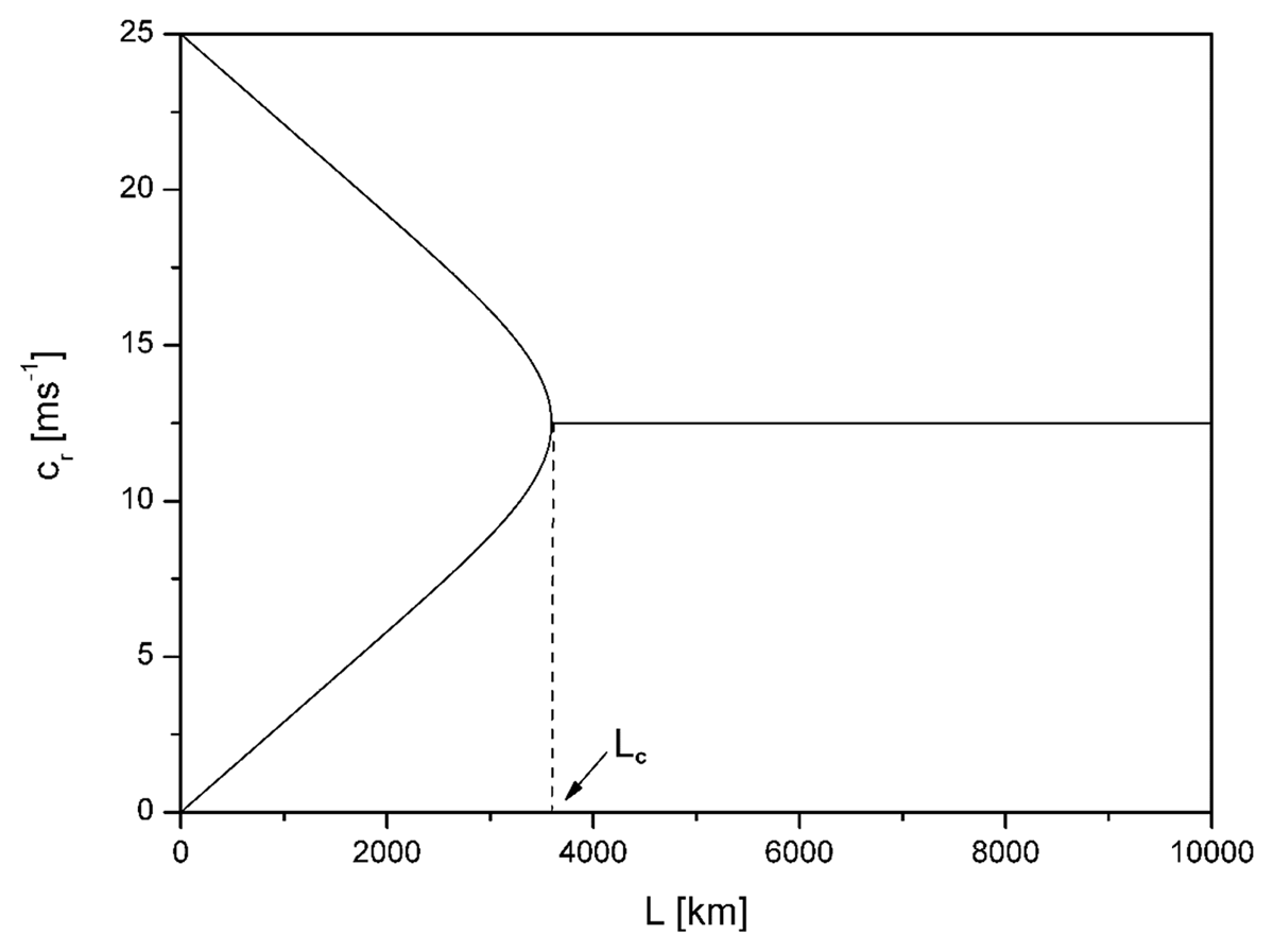
Figure 1
The dependence of the real part of the phase speed cr on the wavelength L of disturbances. Lc denotes the critical wavelength.
From Eq. (25) we also determine the growth rate kci of unstable amplifying perturbations:
The same value of kci, but with the opposite sign, is reached by perturbations whose amplitude decreases with time. The evolution of kci as a function of wavelength is shown in Figure 2. It clearly shows the position of the critical wavelength Lc and that the short-wavelength perturbations are stable, while for L > Lc there are perturbations with increasing amplitude.
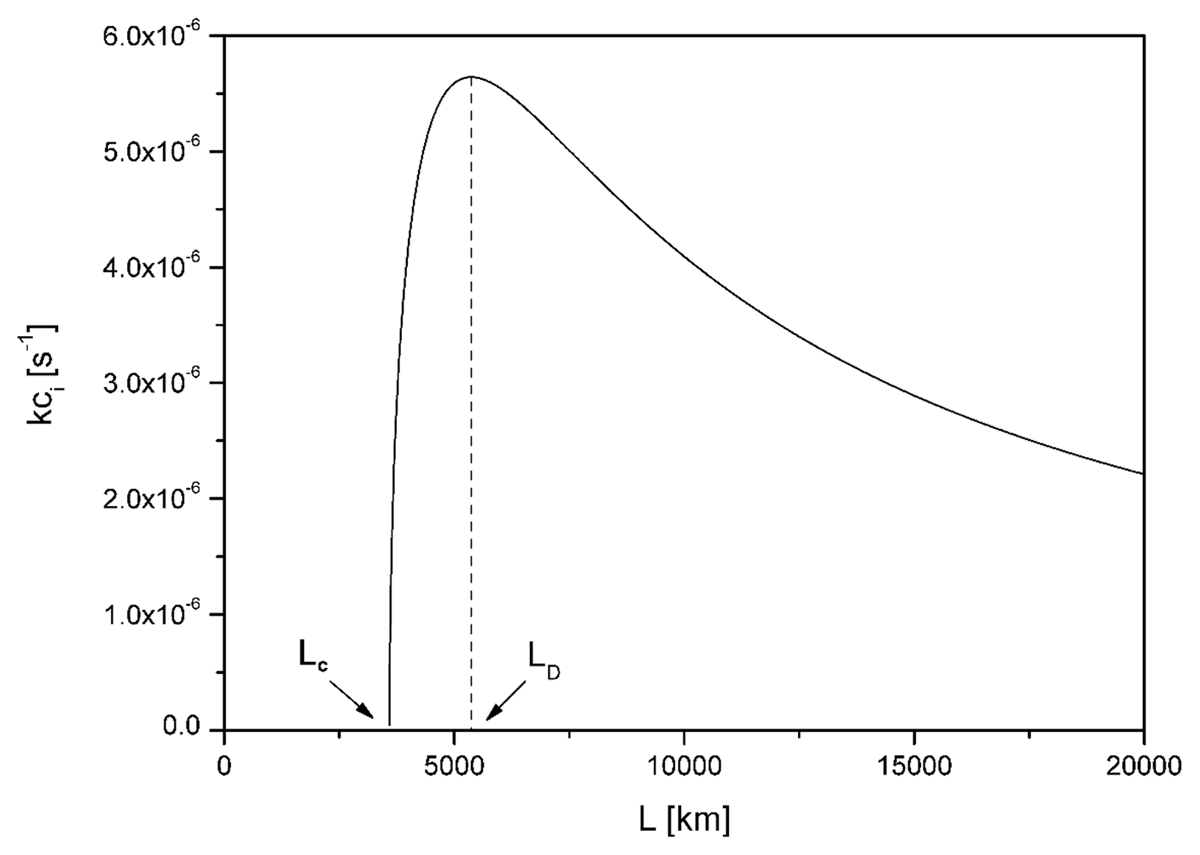
Figure 2
The dependence of the growth rate kci of the perturbations on the wavelength L. LD denotes the wavelength of the dominant perturbation, Lc is the critical wavelength.
Note that there is a wavelength, denoted LD, for which the growth rate is maximum. This means that there is a perturbation that grows fastest in our linear approach and thus starts to dominate the perturbation field after a certain time. This perturbation with wavelength LD will therefore be called the dominant perturbation or disturbance. Figure 2 indicates that growth rate of dominant perturbation is approximately 5.5 ⋅ 10–6 s–1 and the corresponding e-folding time is about 2.1 days. Let us calculate the value of LD. To do this, we need to solve the equation
which, after substitution by Eq. (28) and derivation, leads to the equation
The numerical solution of Eq. (30) gives
from which, after substituting from the Eq. (26b) and using , we obtain the expression for the wavelength of the dominant perturbation:
We used the same values of p0 and f0 in calculating the approximate Eq. (32) as in the calculation of the critical wavelength Lc. By comparing the Eqs. (32) and (27), we see that the wavelength of the dominant perturbation has similar properties to Lc, i.e., it increases with increasing stability of the vertical stratification of the atmosphere and decreases with increasing distance from the equator. After all, as the formulas for LD and Lc show, the two wavelengths are linked by a definite relationship LD ≐ 1.49384Lc. If = 2 ⋅ 10–6m2s–2Pa–2 is selected again, the LD is 5,300 km. As said before, perturbation with this wavelength will dominate the spectrum of increasing perturbations after a certain period, according to the chosen linear approach. If we consider that a quarter of the wavelength of the perturbation corresponds to the distance of the high-pressure ridge from the low-pressure trough, it follows . This agrees very well with the characteristic magnitude of the synoptic-scale disturbances in the midlatitudes. Our model of baroclinic instability thus captures the origin of these synoptic disturbances reasonably well, even within the linear approximation, and with several simplifying assumptions made.
4 Vertical structure of unstable perturbations
4.1 Geopotential perturbations
In the next part of the text, we focus on determining the structure of unstable (growing) perturbations, especially of the dominant perturbation. From Eq. (22a), we express the constant B and substitute into Eq. (19) to obtain an expression for the amplitudes of the perturbation stream function:
However, we are unable to determine the constant A within the framework of linear theory, so in the following we set it equal to one. Keep in mind that the amplitudes obtained can be multiplied by a real non-zero constant, so instead of the last relation we will write
Thanks to Eq. (12), the perturbation stream function can be expressed as
Since we used a simplified relationship between the geopotential and the stream function ϕ = f0ψ, in deriving the potential vorticity Eq. (13), which became the starting point for the present considerations, Eqs. (33) also represent the formulas for the amplitude or perturbation in the geopotential field, except for the multiplier f0:
If we decompose the phase speed of instable disturbances into a real and imaginary part
and if we substitute this decomposition into Eq. (33c), we obtain:
We modify the second term in the square bracket of the last expression as follows:
For the amplitude of the geopotential perturbations, we thus have
and by choosing , where αϕ is the phase angle, we can write
where and further that
Again, recall that only the real part of Eq. (38) is physically meaningful. The vertical plot of the absolute value of the perturbation amplitude in the geopotential field for the dominant disturbance is shown in Figure 3a. We see that the amplitude reaches maximum values at the surface and at the upper boundary of the atmosphere, while it is at its minimum at 500 hPa. The formula (40) shows that for an unstable disturbance the phase angle changes with the vertical coordinate – for a growing perturbation it increases with height, which means that the growing perturbation in the field of geopotential tilts towards the west with increasing height, thus against the direction of the base eastward flow U (see Eq. (18)). In other words, this means that a strengthening perturbation in the geopotential field near the Earth’s surface precedes the perturbation in the higher levels of the atmosphere. This lead depends on the wavelength L > Lc. More detailed calculation can show that for a strengthening wave disturbance with a wavelength of 4,000 km, this lead between the levels of 1,000 and 500 hPa slightly exceeds 20°, while for a disturbance with a wavelength of 7,000 km, the lead is only 10°. Isolines of constant phase satisfy the following relationship at any moment:
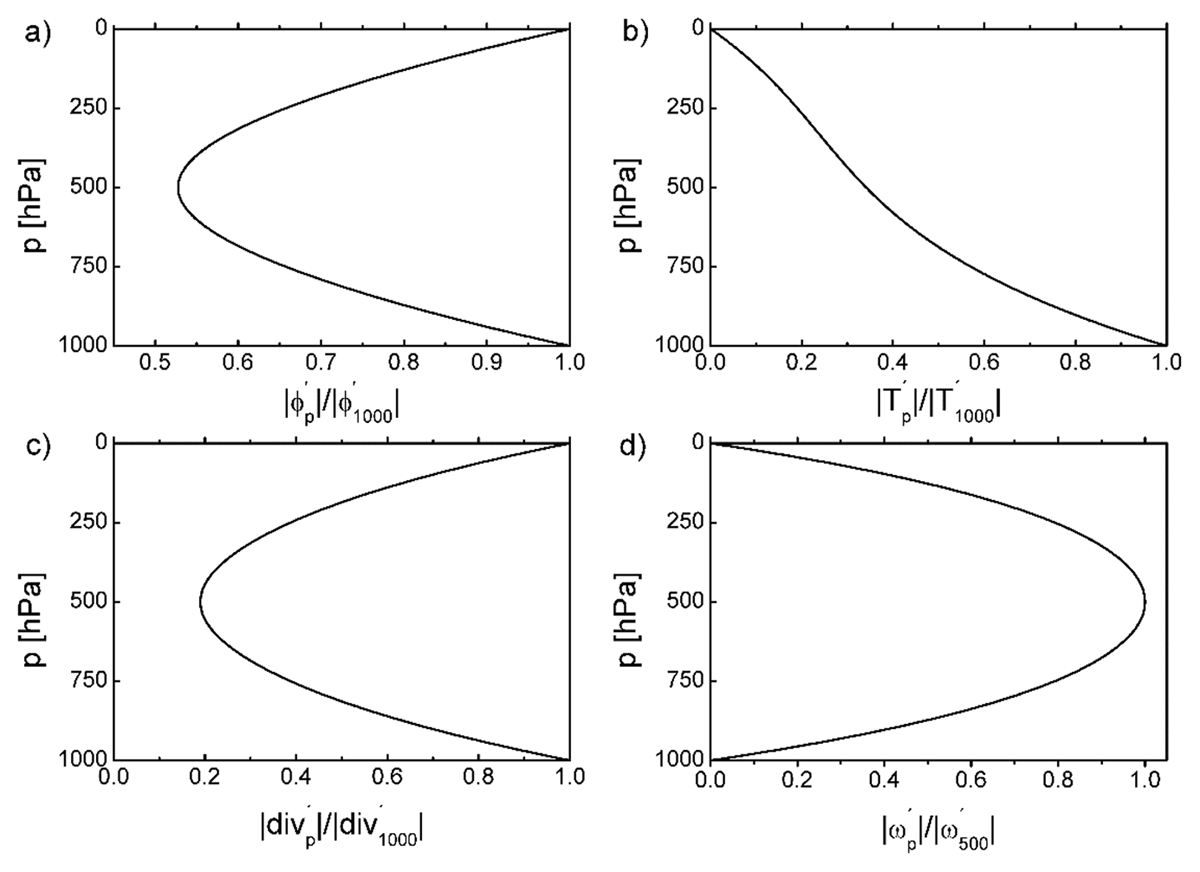
Figure 3
Vertical profile of amplitude of the dominant perturbation in the geopotential (a), temperature (b), isobaric divergence (c), and generalized vertical velocity (d).
The profile of the phase angle αϕ with vertical coordinate for the dominant perturbation is shown in Figure 4a. It is also clear from Eq. (40) that weakening perturbations tilt towards the east in the geopotential field with increasing height, i.e., in the opposite direction to strengthening perturbations.
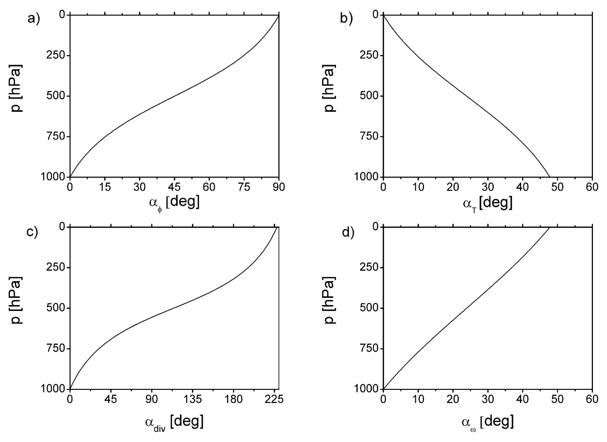
Figure 4
Vertical profile of phase angle of dominant perturbation in the geopotential (a), temperature (b), isobaric divergence (c), and generalized vertical velocity (d).
4.2 Temperature perturbations
Perturbations in the temperature field are determined by the equation of hydrostatic equilibrium
that is
R is the gas constant for dry air, R = 287 J kg–1K–1. By substituting Eq. (34b) into these last Eqs. and using eiπ = –1, we can write
Considering Eq. (34b) it follows that perturbations with time-invariant amplitude are mutually shifted by 180° in the geopotential and temperature fields. If we consider the increasing perturbations and decompose the phase speed c by Eq. (35), we obtain for perturbations in the temperature field
By using a similar procedure as in the expression for ϕ′ (Eq. (38)) we obtain
where
and
Due to the decrease in pressure and air density with height, the amplitude decreases with height, in accordance with Eq. (47) – see Figure 3b. Thus, perturbations in the temperature field are most pronounced at the surface. As for the phase angle, for increasing perturbations this angle αT decreases with increasing height and the isolines of the constant phase in the temperature perturbation field slope towards the east, i.e., in the opposite direction to the geopotential. The vertical profile αT for the dominant perturbation is shown in Figure 4b.
4.3 Isobaric divergence perturbations
Perturbations in the field of isobaric divergence in the p-system, , are determined using the vorticity equation (Eq. (1)), which for perturbations under the given assumptions switches to the form
The continuity equation in the p-system can be expressed as
By combining the last two equations with respect to Eq. (12) and rearranging, we obtain
Using Eq. (35) and analogous modifications as in the derivation of Eqs. (38) and (46) after some calculations we arrive at the expression
where
The vertical profile of the amplitude for the dominant perturbation is shown in Figure 3c. It is clear from this that we observe the minimum, but not zero, divergence at the 500 hPa level. This agrees relatively well with the conditions in the real atmosphere, in which the level of minimum divergence is situated in the vicinity of the 500 hPa. The dependence of the phase angle αD on the vertical coordinate for the given perturbation is shown in Figure 4c. The isolines of the constant phase αD tilt westward with height, so they have the same direction as the perturbations in the geopotential field. The difference is that αD has a larger range than αϕ. The tilt of perturbations in the isobaric divergence field is therefore greater than in the geopotential field. In fact, it is also greater than for perturbations in the temperature field and the generalized vertical velocity ω, as we will see later.
4.4 Vertical velocity perturbations
Let us now describe the structure of the vertical velocities in our model. By substituting into Eq. (15) using the thermodynamic Eq. (16), in which we express , we can give the generalized vertical velocity in p-system in the form
Using Eq. (33b) for the perturbation stream function, expressing Eq. (18), and performing similar modifications as in the derivation of Eqs. (38), (46) or Eq. (52), after some modifications we arrive at the following expression for the generalized vertical velocity:
where
The parameters D1 and D2 are given by Eqs. (56). The vertical profile of the || amplitude for the dominant perturbations is shown in Figure 3d. It shows that the most intense vertical movements are registered at the level of 500 hPa, which, after all, we could infer from the knowledge of the isobaric divergence field distribution. The vertical profile of the phase angle αω for the dominant perturbation can be seen again in Figure 4d. This figure shows that the phase angle increases with height, so the isolines of constant phase in the field of generalized vertical velocity tilt towards the west, i.e., against the direction of the basic zonal flow. We arrive at the same situation as we have observed for perturbations in the geopotential field and isobaric divergence.
5 Vertical cross-section of the dominant perturbation
An illustrative view of the mutual arrangement of the individual fields of geopotential, temperature, isobaric divergence, and generalized vertical velocity of perturbations, for which we derived analytical relationships above, provides information about the position of the extrema of these fields at each pressure level. Extrema in the geopotential and temperature fields are determined using the following conditions:
– maximum:
– minimum:
The arrangement of these extremes for the dominant disturbance is shown in Figure 5a. Realizing that ϕmax, or ϕmin, represents the axis of a high-pressure ridge (or anticyclone), or the axis of a low-pressure trough (or cyclone), respectively, it is clear that the surface area of low pressure represents a warm formation with the warmest zone in its frontal part, while the area of high pressure at the ground surface is a cold formation with the coldest air again in front of its surface axis. With increasing altitude, the warm air approaches the high-pressure ridge and the cold air approaches the low-pressure trough. From the above facts and from Figure 5a, it is therefore clear that the geopotential and temperature perturbation fields are not in phase, but rather the geopotential wave precedes the temperature wave. In the steering level of 500 hPa, this lead is 90°, or 1/4 wavelength.
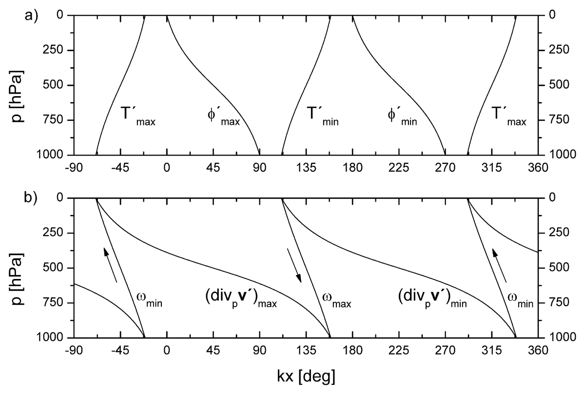
Figure 5
Positions of maxima and minima of the dominant perturbation in the geopotential and temperature fields (a), and isobaric divergence and generalized vertical velocity fields (b).
The profiles of the extremes in the field of isobaric divergence and vertical motion w can be determined in a similar way:
maximum:
minimum:
The configuration of these extremes is shown in Figure 5b. We can see that at the ground surface, the area of minimum isobaric divergence, which is actually maximum convergence is accompanied by maximum upward air motion ωmin, while in the area of the upper atmosphere, the opposite is true – the area of maximum isobaric convergence of flow velocity corresponds to the maximum of downward motion at the upper atmosphere boundary. By analogy, the maximum of isobaric divergence at the surface is associated with the maximum of downward air motions; at the upper boundary of the atmosphere the situation is again reversed, with the maximum of isobaric divergence of the flow velocity coinciding with the maximum region of outward air motions.
Comparing Figure 5a and 5b, we find that in the surface low pressure area, isobaric divergence of the flow dominates along with upward air motion. Note further that the most intense upward air motion is located at the 500 hPa level (see Figure 4d), and at this level the maximum upward motion precedes the surface axis of the low-pressure area by 45°, which corresponds to 1/8 of the wavelength of the disturbance. Therefore, if we hypothetically consider the possibility of water vapor condensation and precipitation, according to our model we would expect the location of the most intense precipitation to be at a distance of approximately ahead of the surface axis of the pressure trough, which for dominant perturbation corresponds to a distance of approximately 660 km.
A comprehensive view of the structure of the most rapidly intensifying perturbation is provided by Figures 6, 7, 8 and 9, which show the perturbations in the geopotential field (Figure 6), temperature (Figure 7), isobaric divergence (Figure 8), and generalized vertical velocity (Figure 9) for one and a quarter wavelengths of the LD. All four figures essentially confirm the previously presented results. At this point, however, it should be pointed out that our temperature perturbations pattern in Figure 7 differs from the isolines of the temperature perturbations published by Holton (2004, Figure 8.10 page 259), who also analyzed the Eady-type model. The Holton temperature perturbations have the same amplitude at the lower and upper boundaries of the model. However, Holton (2004) followed Eady (1949) more closely, in that he constrained the model by two rigid boundaries at heights z = 0 and z = H < ∞ and worked with the height z as the vertical coordinate. In our opinion, our modification of the Eady model and the use of the p-system better corresponds to the conditions in the real atmosphere.
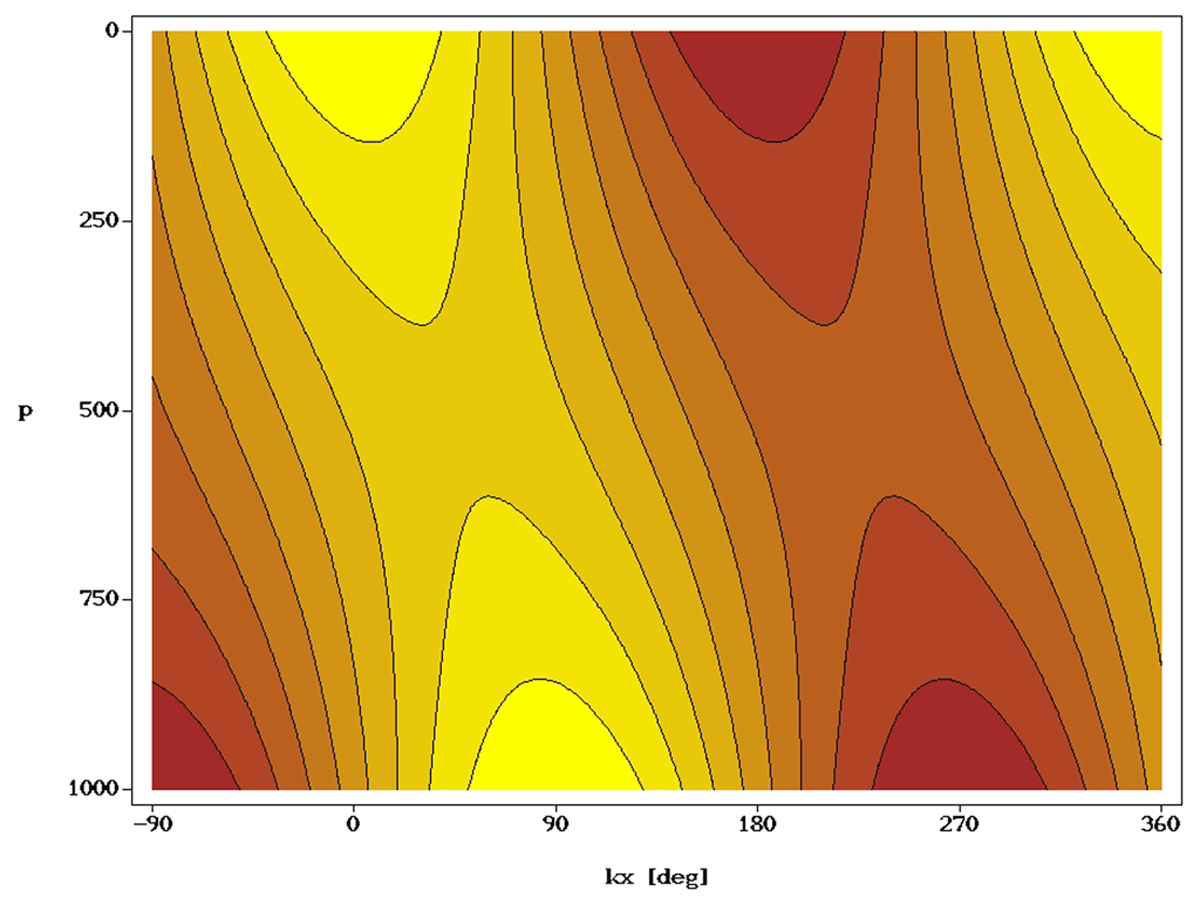
Figure 6
The geopotential field of the dominant perturbation. The high-pressure region is shown in yellow, the low-pressure region in brown.
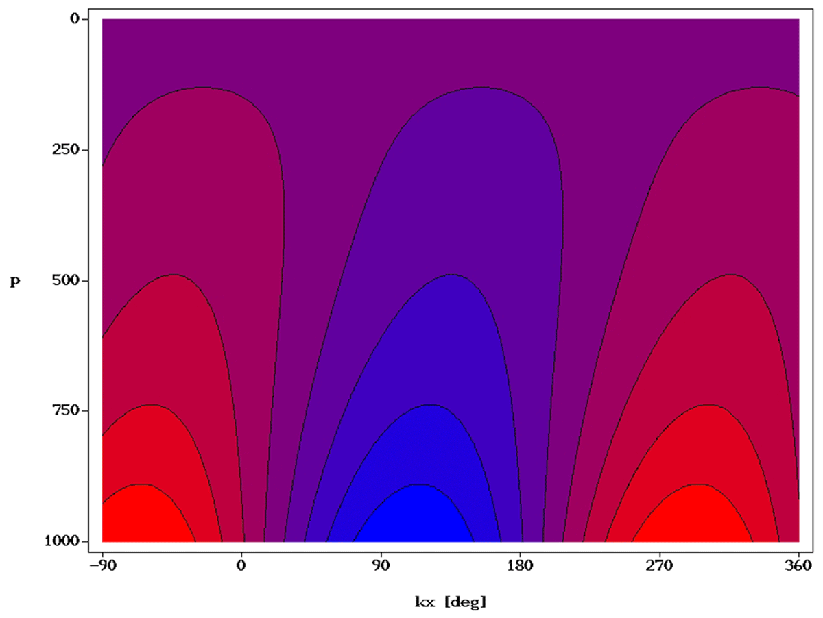
Figure 7
Temperature field of the dominant perturbation. The coldest air region is plotted in blue, the warm air region in red.
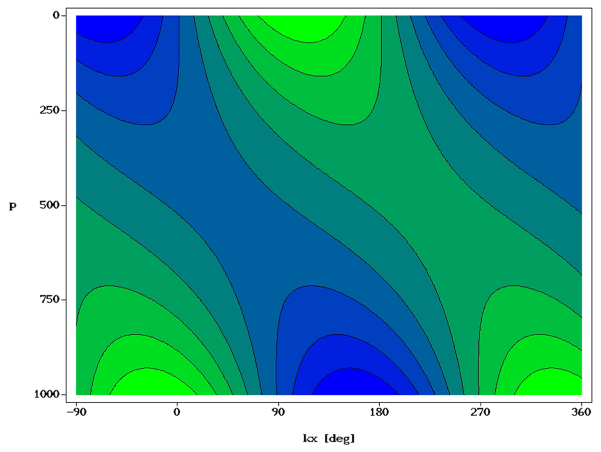
Figure 8
The isobaric divergence field of the dominant perturbation. The region of isobaric divergence is plotted in blue, the region of isobaric convergence in green.
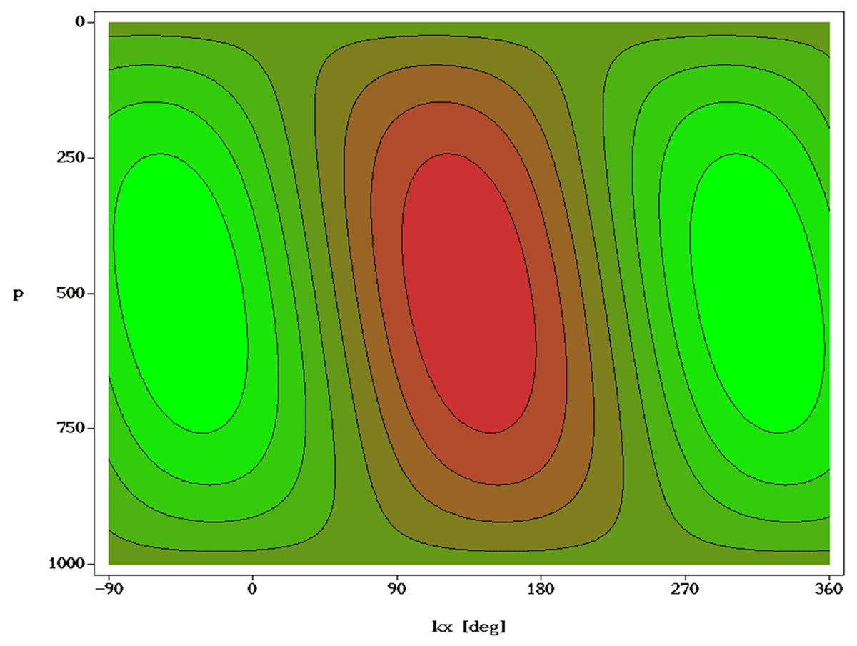
Figure 9
The generalized vertical velocity field of the dominant perturbation. The region of downward motions is plotted in brown, the region of upward motions in green.
Concluding remarks
It was demonstrated that despite using a relatively simple model, we were able to capture some of the key properties of real synoptic-scale disturbances in the midlatitudes, primarily in the early stages of their development, due to the linearization of the governing equations as discussed in section 2. The model only considers perturbations that are sufficiently small compared to the corresponding non-perturbed basic state quantities. Its limitation therefore is that it cannot, in principle, describe the evolution of perturbations of finite magnitude that would evolve due to the nonlinear terms in Eqs. (7) and (14). Even so, the linearized model satisfactorily describes the wavelength of the dominant disturbance and its vertical structure, as well as to the e-folding time. We have also identified relatively well the level of minimum divergence in the region of 500 hPa, as well as the position of the steering level. The simplification applied us to address the problem of baroclinic instability in a strictly analytical way without resorting to numerical approximation. As the above shows, we have largely succeeded in this task. Similarly, using the p-system allowed us to work over the entire range of the atmosphere, and to use the natural boundary conditions at the upper and lower limits of the atmosphere, (whereas typical Eady-type models are formulated so that the upper boundary condition is defined at the upper boundary of the troposphere).
A clear disadvantage of this Eady-type model is the use of the f-plane approximation, i.e., the neglect of the variation of the Coriolis parameter with latitude. This is particularly evident in the instability of very long waves. In models of baroclinic instability that consider the latitude variable Coriolis parameter, for example through the β-plane approximation, very long waves are stabilized.
Potentially, it should be possible to further improve the model and to make it even closer to the conditions in the real atmosphere. If an entirely analytical solution is required, the energetics of and Eady-type model should be possible to incorporate into the framework of linearized equations. We also plan to do this as a part of further research. Separate effort could be devoted to introducing diabatic heating, surface friction, instability of nonzonal flow and/or finite amplitude instability (Pedlosky, 1987), and to other aspects, such as including a more realistic profile of wind speeds at mid-latitudes – some of the climatological reanalysis dataset could be used for this purpose. However, in these cases a strictly analytical approach would no longer be possible, and numerical methods would be required to reach the solutions.
It should also be noted that the normal modes method is not the only way to investigate baroclinic instability. Attention should also be paid to the nonmodal growth of perturbations, the classical concept of cyclogenesis in synoptic meteorology (Lackmann, 2011), or potential vorticity thinking (Holton, 2004).
Since we conclude this paper with an appendix on the choice of the mean value of the static stability parameter, let us also discuss in more detail the effect of the stability of the vertical atmospheric stratification on the growth rate of different long-wavelength disturbances. According to Dymnikov and Filatov (1990), the variation of the stratification in the lower atmosphere between 925 and 855 hPa mostly affects the stability of disturbances with wavelengths around 1,000 km. Stratification changes in mid-troposphere have significant effect on the growth rate of disturbances with wavelength of 2,000 to 3,000 km, but have no effect on shorter disturbances. Changes in the vertical stratification of the atmosphere at its highest levels have only a very weak effect on the growth rate of disturbances of all wavelengths.
Appendix
Let us investigate further the choice of the mean value of the atmospheric static stability parameter . Assuming a temperature gradient in the troposphere and substituting into the definition of the static stability parameter
using the Poisson equation (definition of potential temperature), the equation of state, and the hydrostatic equilibrium equation, we get:
Integrating the last equation, we get
which, after substitution into Eq. (A1), leads to the relation:
where
T0 is the temperature at the pressure level p0 = 1000 hPa. The mean value in a certain region of the troposphere between the pressure levels p1 and p2 is obtained as follows:
Using the last equation, we can easily verify that the value = 2 ⋅ 10–6 m2s–2Pa–2, which we commonly use, represents the mean value of the atmospheric static stability parameter between the pressure levels 1,000 and 350 hPa and the temperature T0 = 288 K at the 1,000 hPa level.
Data Accessibility Statement
The source codes are available from http://www.doi.org/10.17605/OSF.IO/XH6S8.
Competing Interests
The authors have no competing interests to declare.
Author Contributions
A.R. designed the research, performed the calculations and wrote the manuscript. H.B. and J.M. supervised the research, and J.M. finalized the manuscript.