
1. Introduction
Searching for the limit in tropical cyclone (TC) intensity forecast accuracy is a challenging problem in TC research and operation. One key difficulty in studying such TC intensity predictability (TIP) is rooted in an open question of whether TC dynamics possesses chaos at any stage of TC development (Kieu and Rotunno, 2022; Kieu et al., 2022). For practical purposes, a TC intensity forecast must be issued from an early formation to the final dissipation stage, yet all current predictability frameworks require a stationary attractor or fully-developed turbulent state such that statistical properties can be well-defined (e.g., Lorenz, 1963; Lorenz, 1969; Leith, 1971; Métais and Lesieur, 1986; Vallis, 2017). This fundamental requirement of stationary statistics for chaotic dynamics explains confusingly different estimations for TIP, which varies from 3 hours to 7 days in previous studies (Hakim, 2011; Hakim 2013; Emanuel and Zhang, 2016; Kieu and Moon, 2016; Judt et al., 2016; Zhong et al., 2018).
Of all TC development stages, the only one that appears to meet the requirement for chaos analyses is the maximum intensity state, known as the TC potential intensity (PI) (Emanuel, 1986; Emanuel, 2003). According to the PI theory, TCs will reach a steady state with a maximum intensity determined by environmental conditions. The existence of this PI state and its related stability have been extensively studied in previous observational, theoretical, and modeling studies (e.g., Bryan and Rotunno, 2009; Hakim, 2011; Kieu and Wang 2017; Kieu, 2015; Rotunno and Emanuel, 1987). However, whether a PI limit truly exists is still inconclusive, as several modeling studies, e.g., by Smith et al. (2014; 2021) or Persing et al. (2019) showed that a TC vortex cannot maintain a steady state due to the transport of low angular momentum from upper levels to the surface. This process cuts off the supply of high angular momentum from the outer-core region and eventually weakens TC intensity, even under idealized environments.
Despite the controversial existence of the PI state, the fact that the maximum TC intensity can be captured and well maintained in very long integrations (e.g., Brown and Hakim, 2013; Hakim, 2011; Kieu et al., 2022) suggests that TC dynamics can settle down in a quasi-stationary equilibrium if proper experiments are designed. Such an equilibrium, hereinafter referred to as the PI equilibrium, offers a unique opportunity to quantify TIP in accordance with the current chaos theory. Specifically, the PI equilibrium helps define a reference climatology for TC intensity, on which one can measure error growth over time. The range of predictability is then the maximum time interval at which a forecast distribution of TC intensity becomes indistinguishable from its climatology. Given a measure for such an intensity difference between the forecast and climatology distributions, a predictability range can be then obtained by using, e.g., the decorrelation time, integrated time, or signal-noise ratios as studied in, e.g., DelSole and Tippett (2007; 2009), Lorenz (1969); Shukla (1981).
Taking advantage of such a PI equilibrium in model simulations, Kieu and Moon (2016) presented a method to quantify TC intensity chaos based on a fidelity-reduced model proposed by Kieu (2015). Using TC scales obtained from a long integration of Rotunno and Emanuel (1987)’s axisymmetric model as dynamical variables, Kieu and Moon (2016) demonstrated that TC intensity appears to approach a chaotic region in the phase space constructed from a few basic TC scales. In this phase space, PI is no longer a single point but a bounded region with all the properties of a typical chaotic attractor. A direct implication of this chaotic PI attractor is that TC intensity must possess some intrinsic variability, even for a perfect TC model under ideal conditions.
Of further importance about the existence of such a chaotic attractor is that TC intensity, once settling down in the PI equilibrium, should have limited predictability. The current estimation for TIP varies widely due not only to the dependence of PI on specific model dynamics, ocean basin, or environmental conditions, but also to how one defines a reference climatology for TC intensity. This uncertainty in estimating TIP is especially challenging for real TCs, because real TCs constantly move from one environment to the next that they may have no time to reach their PI (e.g., Keshavamurthy and Kieu, 2021; Kieu and Moon, 2016), thus preventing one from quantifying TIP reliably.
Despite such an inconclusive range for TIP, the potential existence of low-dimensional intensity chaos is itself important from several angles. First, this low-dimensional attractor helps justify why forecasters can use only a few bulk numbers such as the maximum surface wind (Vmax), the minimum central pressure (Pmin), cloud top temperature, or storm size to characterize a TC, instead of all possible details about TCs. This is also consistent with the fact that TC intensity models with only a few degrees of freedom could capture some broad properties of TC intensity as shown in previous studies (e.g., Emanuel, 2003; DeMaria, 2009; Schonemann and Frisius, 2012; Kieu, 2015; Wang et al., 2021).
Second, the existence of low-dimensional chaos indicates that PI should not be represented by a single Vmax value as in the current PI framework. Instead, the maximum intensity that a TC can get must vary within a range around the PI equilibrium, regardless of how perfect an environmental condition or a TC model is. As a result, this intrinsic variability of TC intensity will act as a “noise” level in any TC intensity statistics that one has to take into account when projecting any change of PI under different climate conditions.
Third, the PI equilibrium is no longer just about Vmax. Instead, PI has to be characterized by other features as well such as the warm core anomaly, the maximum radial wind (Umax) in the boundary layer, the radius of maximum wind (RMW), or the maximum eyewall vertical motion (Wmax). Therefore, any factor that can influence other dimensions of PI would cause strong fluctuation in TC intensity, regardless of whether Vmax is equal to PI or not as discussed in Kieu (2015).
While both idealized simulations and real-time forecast verification strongly hint at a possible existence of TC intensity chaos, examining this intensity chaos and the related TIP turns out to be difficult due to the various ways that one can define a reference climatology for TC intensity in practice. Note again that predictability is not a universal measure, as it must be associated with one specific variable over a specific period during which a reference climatology is constructed. Thus, predictability can be different for different intensity metrics. Because of this metric dependence, any estimation of TIP must be tied to a specific intensity metric and its climatology.
Given such important implications of intensity chaos and the uncertainty in estimating TIP, a better understanding of TC intensity chaos is needed so that a more accurate range for TIP can be obtained. In the next, we will present our examination of TC intensity chaos within a framework of deterministic chaos, which is suitable for point-like intensity metrics such as Vmax or Pmin. Details of our machine learning (ML) approach for chaotic systems are provided in Section 2. Section 3 presents the details of ML models, followed by the main results in Section 4 and concluding remarks in Section 5.
2. Methodology
2.1. Maximum intensity equilibrium
If the PI equilibrium is the only possible state of TC development whose statistical properties are stationary for intensity climatology, how can we use this equilibrium to examine TC intensity chaos? In this study, we will follow the same approach as in Kieu et al. (2022) and assume that the PI equilibrium can be characterized by a low-dimensional phase space where chaos manifests. Note that Kieu et al.’s approach based on the phase-space reconstruction method to directly search for the dimension of a chaotic attractor contains significant subjectivity and is sensitive to data noise (e.g., Kantz and Schreiber 2003). Here, we propose to use ML to quantify the TIP range, which can also confirm the existence of TC intensity chaos, albeit less directly as compared to the phase-space reconstruction method.
A key part in searching for chaos at the equilibrium is therefore to obtain first a statistically stable PI state so that one can analyze it. Given such a state, one can then extract the time series of key TC scales such as Umax, Vmax, Wmax, or Pmin, which can serve as input features for ML training. Details of a long simulation of TC intensity that ensures such a stable PI state and how to extract the required data for the ML approach will be given in Section 3, which are identical to those used in Kieu et al. (2022).
2.2. Machine learning approach
Broadly speaking, machine learning (ML) can be considered as a framework that can search for rules from data. Given an ML architecture, a measure of accuracy, and input data, the rules can be obtained within a prescribed level of accuracy. The key advantage of ML in practical applications lies in its ability to learn rules from input data without a priori knowledge, provided that the input data is sufficiently good (i.e., the input data can ensure several criteria including i) comprehensiveness, ii) relevancy, ii) consistency, and iv) uniformity.) With an inherently large volume of data, climate and weather prediction provide a great domain for ML applications, which justifies the surge of ML applications in atmospheric science recently.
Specifically for TC intensity, ML offers a unique way to study low-dimensional chaos. To set up a context for applying ML to our TC intensity chaos problem, we will focus hereafter on supervised ML, which requires a set of input data and corresponding targets (labels) for training an ML model. At a basic level, supervised ML models need a surjective mapping between an input training dataset and a target dataset (i.e., one will have at least one ) so that the training can be carried out. For a typical time-prediction problem (i.e., given a state of a system at one time t = 0, one needs to predict the state of the system at a later time ), this mapping can be considered as a propagator from a given initial condition to the later time . Mathematically, such a propagator can be expressed as , where is the propagator from t = 0 to and x(t) is the model state at time t.
For a full-physics model, is nothing but a numerical model with governing equations integrated from t = 0 to . For ML, is a however nonlinear operator that is learned from a training dataset. In principle, the more data we have, the better an ML model can search for underlying rules and build without any physical equations. Thus, we can feed an ML model with a large amount of data, and let it figure out the best possible relationship between t = 0 and . For deep learning that is based on neural networks, an ML model with sufficient layers and depth should capture a nonlinear mapping between two time slices, making it suitable for TC intensity prediction.
From this perspective, it is immediate that chaotic systems will pose a challenge to any ML model, because one input may give totally different outcomes after reaching predictability limit T (i.e., one would give two different , where two input x1, x2 are practically considered to be the same as x if their difference is within some measurement errors, for a sufficiently small uncertainty ϵ). So, there exists no longer a good mapping between the training and the label datasets, and ML models cannot learn any rule from data.
The deterioration of ML models after entering the chaotic regime as described above suggests, however, a unique way to study chaotic systems. Specifically, we will search for a lead time T beyond which an ML model can no longer be trained from any input dataset, which gives us a direct estimation of the predictability range for a chaotic system. This approach is natural in the sense that an ML model should generally be able to predict the next state of a system from a given input, if the system remains predictable and sufficient training data is provided. As soon as the system enters a chaotic regime, ML models are no longer trainable. From this perspective, ML models are naturally a great tool for studying chaos.
Our aforementioned use of ML to examine predictability is well suited for TC intensity, as this approach serves two purposes: i) it verifies if a low-dimensional representation is sufficient for TC intensity, and ii) it helps estimate the TIP range in that low-dimensional phase space. Our underlying hypothesis is that an ML model can predict TC intensity in a low-dimensional phase space, whose dimensions correspond to several basic TC scales, up to a certain lead time T. Beyond this lead time T, ML models can no longer be trained to predict TC intensity, thus revealing TC low-dimensional chaos and providing us an estimation for TIP.
The results in Kieu et al. (2022) provide a pathway to verify this hypothesis with ML. Specifically, we will assume that TC intensity can be described by four dimensions corresponding to four TC scales including Vmax, Umax, Wmax, and Pmin. While it is not known in advance the exact dimension of the PI attractor, Kieu et al. (2022) suggested that a minimum dimension of 4 should be sufficient to capture TC intensity chaos within the deterministic framework. As such, we will treat these four dimensions as input features for several ML models to be presented in Section 3b. With these ML models, we can examine how they forecast intensity at different lead times and estimate the TIP range as expected.
3. Experimental designs
3.1. CM1 model configuration
In this study, the same axisymmetric configuration of the Cloud Model (CM1) (Bryan and Fritsch (2002) was used as in Kieu et al.’s study (2022), which produces a quasi-stationary PI state during a long integration of 100 days. This model configuration has 360 grid points on a stretching grid in the radial direction, with the highest resolution of 2 km in the vortex’s inner core region and stretched to 6 km in the outer core region. Unlike the radial direction, the model was configured with 61 levels in the vertical direction, with a fixed resolution of 0.5 km. This fixed vertical resolution was found to be more numerically stable and also less restrictive when choosing the number of vertical levels. In addition, we applied the open-radiative lateral boundary conditions option to the radial direction, and free (no) slip boundary to the top (bottom) boundary in our simulation. The model was initialized from the tropical Jordan sounding on an f-plane, with fixed sea surface temperature (SST) = 302.15 K.
Similar to the results in Hakim (2011) and Kieu and Moon (2016), a long simulation of a quasi-stationary TC intensity with the CM1 model would require a proper choice of model physics to avoid the gradual change in TC environment inside a box domain, which can cause decaying due to the transport of low angular momentum in the outer core region. A simple treatment for this environment change is to apply a fixed Newtonian cooling relaxation of 2 K day-1, as in Kieu et al. (2022), which can result in a quasi-stationary maximum intensity equilibrium in the CM1 simulation for 100 days. Along with this radiative forcing, a suite of other physical parameterizations were also used, which include the YSU boundary layer scheme, the TKE subgrid turbulence scheme, and the explicit moisture Kessler scheme with no cumulus parameterization.
With the PI equilibrium in our 100-day simulation established, the model was then output at every time step of 36 seconds, producing a dataset of length . All time series of four major TC scales including Vmax, Umax, Wmax, and Pmin were extracted from the model output and further split into three subsets for ML training—the training, validation, and test sets with a ratio of 90%, 5%, and 5%, respectively. To ensure that all data are selected at the PI equilibrium, the first 10 days of simulations were discarded. Other details of this CM1 100-day simulation can be found in Kieu et al. (2022), and so we do not repeat them here.
3.2. Deep-learning models
Given the low dimensionality of feature vectors used for our ML training, we present in this study several deep-learning models for TC intensity prediction. Specifically, three popular ML architectures including a deep neural network (DNN) model, a gated recurrent unit (GRU) model, and a long-short term memory (LSTM) were implemented. The applications of these deep learning models in the weather domain have been rapidly growing due to their capability as well as the availability of computational resources, which help accelerate their execution for practical problems. With four TC scales as input features and one real-value output Vmax representing TC intensity, predicting TC intensity with the above ML models thus becomes a familiar supervised regression problem for which these ML models fit very well.
For our TC intensity prediction with DNN, a simple design of 3 hidden layers with layer sizes of 32, 64, and 64 was used, followed by an output layer of size 1 that corresponds to Vmax. Each neural layer was applied a standard ReLU activation, which helps ML models capture nonlinear effects and increase the interaction among layers. One could certainly design a deeper neural network for a more complex relationship between input and output layers. However, our experiments with different DNN designs showed very little improvement for more than 3 hidden layers when predicting TC intensity in a low-dimensional input space. As such, a fixed design of 32, 64, and 64 nodes was used.
For LSTM and GRU, these are recurrent neural models that further require a data interval in the past to capture the memory in the training data. Our model architectures for these LSTM and GRU models thus need some additional setup. Specifically for these recurrent network models, we used a range of time slices, i.e., , as input for LSTM/GRU models when predicting TC intensity at any given lead time. Here, M determines the number of time slices in the past that are needed for recurrent networks, which varies from 5–20 in this study. To avoid overfitting during the training process, we also used three layers of size 16, 32, and 64, with a dropout rate of 0.5. Technically, dropout is a type of regularization that can help reduce overfitting in ML models. There is no particular formula to choose the value for this hyperparameter, other than empirical trials. For our intensity chaos problem, this dropout turns out to be important to ensure good model performance.
All of these ML models employed the mean absolute error (MAE) metrics for the accuracy and the root mean squared errors for the loss function, with a fixed number of training epochs set to be 200. The standard optimizer for the gradient search based on the stochastic mini-batch learning method, the so-called Root Mean Squared Propagation (RMSprop), was applied to all training. Because of the different scales of the wind and pressure variables, all input data was normalized by the standard deviation around their mean value, which corresponds to the PI state of the model vortex at the quasi-stationary equilibrium.
4. Results
4.1. Predictability limit on attractor
Given the current definition of TC intensity in terms of the maximum 10-meter wind, we examine first TC intensity chaos using Vmax as a metric for TC intensity in our ML models. Recall here that, if TC dynamics possesses chaos at the PI equilibrium, then TC intensity should have a limited predictability range that dictates the value of TIP. Thus, a finite TIP range can serve as a proxy for the existence of TC intensity chaos that we are searching for.
In this regard, Figure 1 shows the training absolute mean error as a function of epochs (iterations) for three models at three forecast lead times including 3 minutes, 1 hour, and 3 hours. One notices indeed that the training errors rapidly decrease for minutes in all three ML models (black curves in Figure 1), reaching a relative minimum error of ≈ 0.05, 0.12, and 0.22 for LSTM, GRU, and DNN models, respectively. Looking at the correlation between the ML forecast and the true TC intensity for the test data in Figure 2 (red points), it confirms that all ML models could predict very well TC intensity variability for the short lead time minutes in the 4-dimensional phase space. This result is noteworthy, because these ML models require a minimum number of input features, yet they could produce a good forecast of TC intensity based solely on training data. From this perspective, Figures 1 and 2a help confirm that a low-dimensional phase space suffices to predict TC intensity variability at least for a short lead time, without any physical or governing equations.
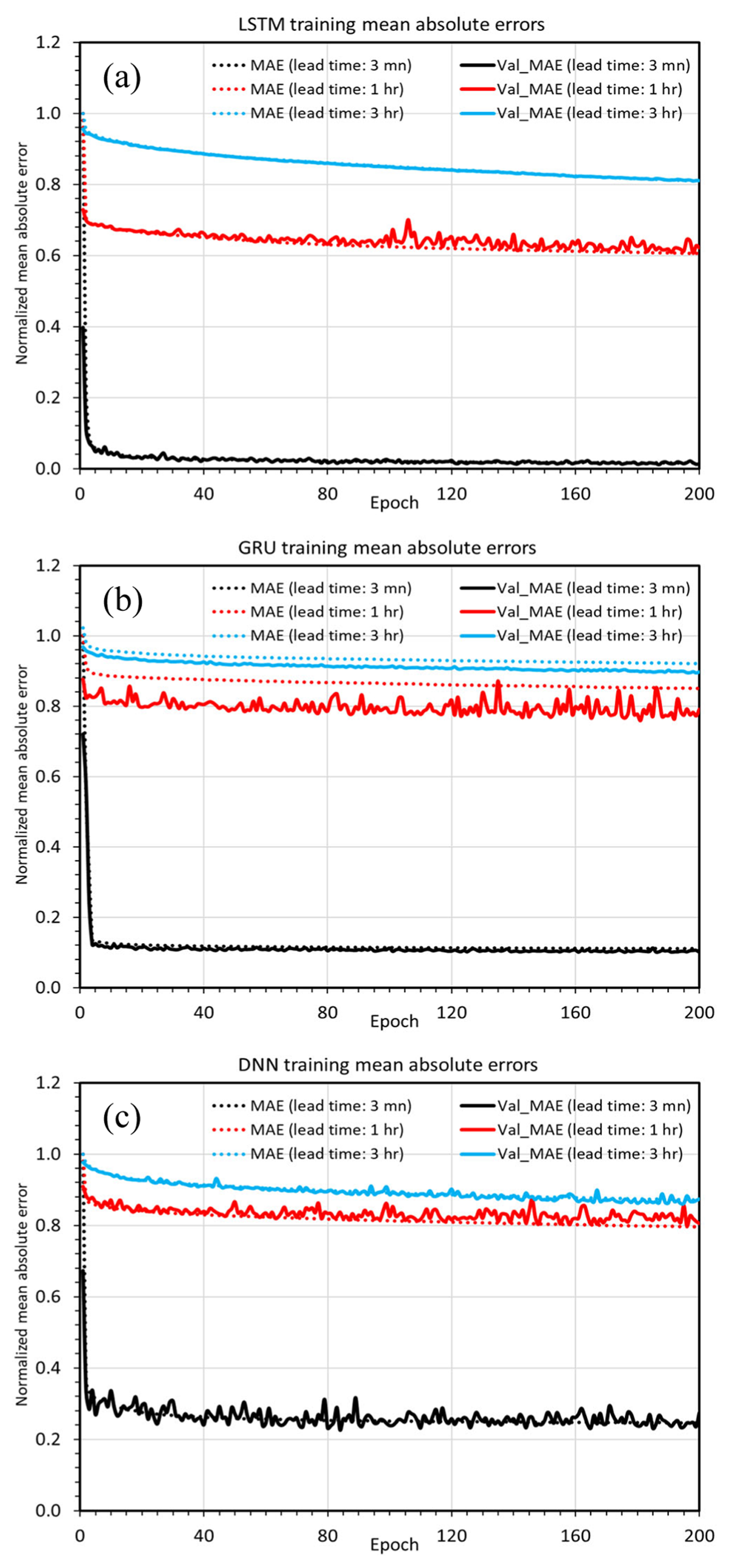
Figure 1
ML accuracy metric based on the mean absolute error (dotted lines) during the training process as a function of iterations (epochs) for three different ML models a) LSTM, b) GRU, and c) DNN at forecast lead times of minutes (black), 1 hour (red), and 3 hours (blue). All absolute errors are normalized by the errors at the first iteration (epoch 1) for better comparison among different lead times. Solid lines denote the mean absolute errors for the corresponding validation dataset in each training process, and the recurrent timesteps M = 5.
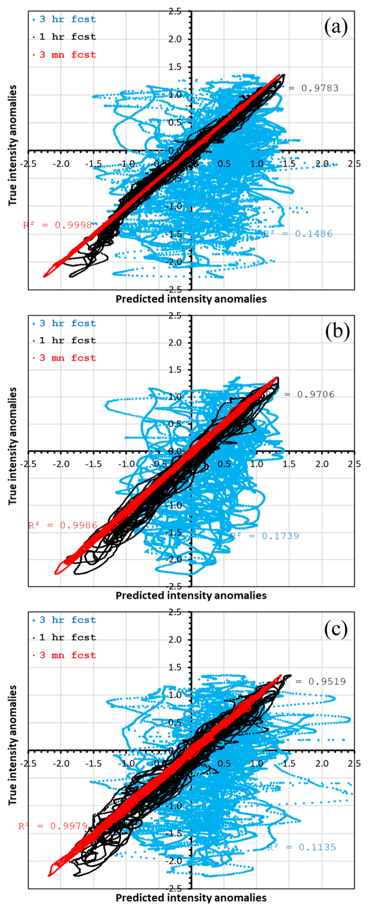
Figure 2
Scatter plots of the ML-predicted TC intensity anomaly (x-axis) and the CM1 true intensity anomaly (y-axis) for a test dataset taken between t = 90–100 days of the CM1 simulation at three lead times: minutes (red), 1 hour (black), and 3 hours (blue) for a) LSTM, b) GRU, and c) DNN model. Note that TC intensity anomaly is relative to the average PI value of 84 ms–1 and normalized by its standard deviation . The R values for each lead time best fit are also provided in each panel.
At the 1-hour lead time, Figure 1 (red curves) shows, however, that all three ML models start losing their ability to be trained quickly. By 3 hours (blue curves), all ML models can no longer be trained, with their errors roughly the same ≈75–85% relative to the initial error value during the entire training period no matter how many epochs are used. Their predictions for the test set at the 3-hour lead time display almost completely no correlation to the true intensity (Figure 2, blue dots). This result reveals that hrs is the longest lead time that these ML models can predict TC intensity at the PI limit. It is of interest is that this estimation is also consistent with the estimation from attractor invariants based on a leading Lyapunov exponent and the Sugihara-May correlation in Kieu et al. (2022), which showed that TC intensity loses predictability in just ≈3–6 hours as soon as TCs reach their PI equilibrium.
The dependence of these ML-based intensity predictions on forecast lead times is best seen when we compare these predictions to a reference (or climatology) forecast, which is taken to be a simple average of Vmax at the PI equilibrium. Figure 3a shows the forecast skill of three ML models relative to this reference forecast as a function of lead times. It is apparent from Figure 3a that ML models perform best for hours. Beyond this, the ML-based prediction skill is no better than a simple forecast using just the averaged Vmax at the PI equilibrium. This short predictability is further supported by the error growth curve (Figure 3b), which displays a typical behavior of chaotic systems with rapid error growth during the initial period and reaching a saturation level after ≈ 3 hours.
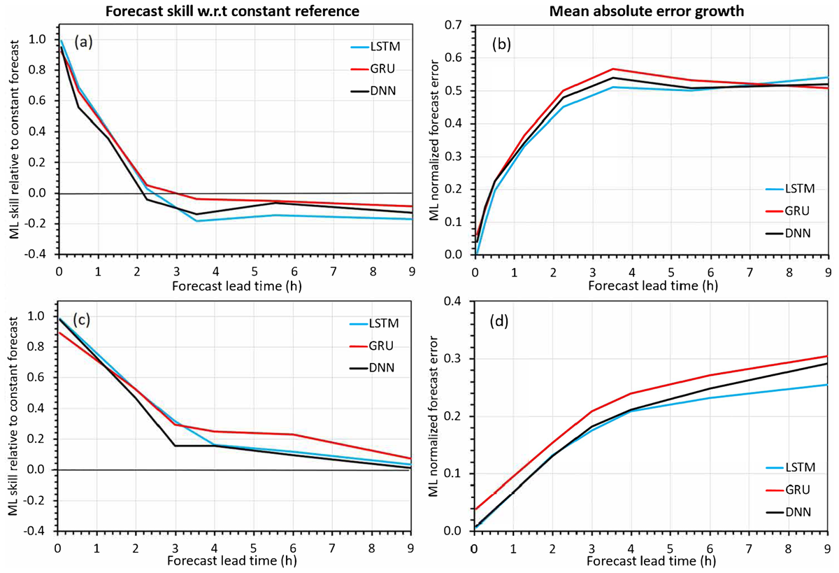
Figure 3
a) Forecast skill of three ML models LSTM (blue), GRU (red) and DNN (black) as a function of lead time relative to the reference forecast that uses the average Vmax value at the PI equilibrium, and (b) similar to (a) but using Pmin for TC intensity. Here, the forecast skill is defined as 1-MAEML/MAEref), where MAEML and MAEref are the mean absolute errors from the ML predictions and reference prediction of TC intensity over the test dataset, respectively.
We emphasize that the decaying of the ML-based forecast skill with does not hold true for any system. In fact, a simple experiment using purely random data as an input for ML training would result in zero forecast skill at all lead times (not shown). This is because the information from one time step does not have any influence on the next, and so ML models cannot learn anything. On the other hand, for completely periodic systems, the forecast skill will always take a constant value of 1 for all lead time as discussed in, e.g., Sugihara and May (1990). As such, the decaying curve of the forecast skill or the error growth curve shown in Figure 3a–3b is an inherent characteristic of chaotic systems, which is captured by our ML models.
Given the average Vmax = 84 ms–1 with a standard derivation is ≈7.5 ms–1 at the PI equilibrium, the TIP range obtained from Figure 3a implies further that TC intensity must vary indistinguishably within an interval of 84 ± 7.5 ms–1 after just 3 hours, even for a perfect TC model. This TIP range may even be shortened if stochastic forcings, asymmetric processes, or model internal errors are taken into account as discussed in Nguyen et al. (2020) or Kieu et al. (2022), which are, however, beyond the scope of our study here. Despite these issues, the results obtained from our ML models herein can at least advocate the existence of intrinsic variability of TC intensity due to chaotic dynamics, which prevents the absolute intensity errors in any TC models from being reduced to zero.
Among the three ML models, it should be mentioned that LSTM and GRU appear to perform best in terms of either the training/validation mean errors due to their use of extra past information (Figure 1–2) or forecast skill (Figure 3a). This past information contains some temporal relationships that help improve future prediction. Thus, LST/GRU presents a very different way of forecasting as compared to the traditional approach based on physical principles. To some extent, recurrent networks improve their prediction in the same way that four-dimensional data assimilation optimizes an initial condition over an interval instead of just a single time slice. Despite this extra information from the past, the predictability of Vmax could not be lengthened beyond 3 hours in both LSTM and GRU models as shown in Figures 2, 3.
4.2. Metric dependence
Because predictability is metric-dependent, an apparent question is how the estimation of TIP changes when using Pmin for TC intensity instead of Vmax. In this regard, Figure 3c–d shows the ML-based forecast skill and error growth curve for Pmin as a function of lead time for three ML models, similar to Figure 3a–b. It is of significance to observe that all models could again capture similar decaying of the Pmin forecast skill, but with a significantly slower rate and thus a longer TIP range of ≈8–9 hours as compared to 2–3 hours for Vmax. Such slower decay of the Pmin forecast skill in Figure 3c well accords with slower error growth and a longer time to reach the error saturation as shown in Figure 3d, similar to what was obtained from the phase-space reconstruction method in Kieu et al. (2022).
The fact that these ML models capture such a different predictability range between Vmax and Pmin is intriguing. Recall that Vmax and Pmin are highly correlated in terms of temporal variability due to their pressure-wind relationship. However, Pmin represents the total mass at the storm center while Vmax fluctuates more vigorously due to fine-scale processes at each model grid point. As such, Pmin tends to better display a slow component of TC dynamics, which ML models could somehow detect even when training data contains strong fluctuations from the wind field. From this standpoint, using Pmin for TC intensity could lengthen the range of intensity predictability for operational forecasts as previously noticed (e.g. Kieu et al., 2022; Klotzbach et al. 2020; Magnusson et al., 2019).
Regardless of intensity metrics Vmax or Pmin, the above results reiterate the finite range of TIP as obtained from different ML models. Such a finite range is in fact held for all TC scales that we have examined, not just Pmin or Vmax. Hence, the existence of low-dimensional chaos of TC dynamics as captured in our ML models is well supported, even though we do not currently know any mathematical model that can describe this chaotic dynamics of TC intensity in a low-dimension phase space. In particular, the existence of TC intensity chaos derived from this TIP information confirms that a part of intensity variability in TC models must be inherent to TC dynamics, which cannot be removed from model outputs simply by improving the model physics or initial conditions.
4.3. Sensitivity experiments
To further address the robustness of our results, this section presents some additional experiments in which more input features, different recurrent windows M, and a coarser sampling frequency (30 minutes) for input training data are used. Note that these sensitivity experiments cover just a small part of possible sensitivities that one can examine. For example, one can design deep neural networks with an arbitrary number of layers, nodes, dropout rates, or data augmentation. Within the scope of this study, we will however limit our sensitivity experiments to several key experiments, which suffice to highlight the important points that we want to present herein.
Figure 4a–4b show the forecast skill and the error growth of Vmax for the first group of sensitivity experiments for which the recurrent timesteps M = 5, 10, 20 at a sampling frequency of 30 minutes. Recall from Section 3.2 that M determines how many time slices in the past up to a present time t will be used to predict the future state at . Thus, a larger M (i.e., a longer window of past information) would allow for more input information, and should increase the forecast skill of ML models.
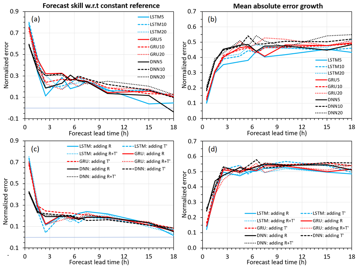
Figure 4
Similar to Figure 3a–3b, but for sensitivity experiments using (a)–(b) different past windows M = 5 (solid), 10 (dashed), and 20 (dotted); and (c)–(d) adding new input features including the radius of maximum wind (R) and the warm core anomaly (T’).
As seen in Figure 4a–4b, forecast skill in these sensitivity experiments all decays quickly during the first 3 hours across the models and recurrent window M, similar to the control settings in Figure 3a–3b. For each model, note however that the longest window M = 20 (dotted line in Figure 4a) appears to be slightly more skillful as compared to the shorter ones, which can be seen in all models. This indicates that longer input windows for recurrent models appear to help improve a forecast skill for chaotic systems, albeit marginally.
The most significant change in these sensitivity experiments is, however, a small but persistent skill of all ML models relative to the reference forecast, even at long forecast lead times hours (Figure 4a). Such a marginal skill is due to the coarser sampling frequency of input data, which eliminates fast fluctuation in the training data and results in some skill relative to the constant reference forecast. From the error growth perspective, it is seen however that there is no significant change in the time needed for the model forecast error to reach its saturation (Figure 4b). All ML models display the same error growth saturation after ≈3 hours, which is an intrinsic property of a chaotic system and independent of how reference forecasts are defined.
Our sensitivity experiments with more input features capture a similar behavior of the error growth and forecast skill as in the recurrent time window experiments (Figure 4c–4d). Specifically, adding more features such as RMW, warm core anomaly (T’), or both does not improve the TIP range. That is, both forecast skill and error growth show rapid decay/increase during the first 3 hours and then approach a saturation limit afterward. This result supports the existence of low-dimensional chaos for TC intensity in the sense that more dimensions in the phase space will not help improve any estimation of attractor invariants as discussed in Kantz and Schreiber (2003) or Kieu et al. (2022). The consistent TIP estimation among ML models and sensitivity experiments as shown above, therefore, confirms the robustness of our finding about the existence of low-dimensional chaos for TC intensity.
5. Conclusion
In this study, we presented a different use of ML to search for chaos in TC intensity. Our underlying assumption was based on the premise that TC intensity at the PI equilibrium can be characterized by a low-dimensional phase space. By treating the dimensions of TC intensity attractor as input features for ML training, the skill of ML prediction can be estimated as a function of forecast lead times. The maximum lead time that ML models can no longer provide skillful TC intensity prediction dictates the range of intensity predictability, which is 2–3 hours as obtained from our axisymmetric CM1 simulation under a fixed environmental condition. The predictability range could be lengthened up to 8–9 hours if the minimum central pressure is used for TC intensity instead of Vmax, yet the limited predictability for TC intensity is still observed in all ML models and sensitivity experiments. As a result of this finite predictability limit, the existence of TC intensity chaos within an idealized environment is established.
While a finite TIP range could reveal the existence of TC intensity chaos, we emphasize that the practical application of such a TIP range for real TC intensity forecast is very limited. This is because the practice of TC intensity forecast requires the prediction of TC intensity from the very early development of a TC to the final dissipation stage. At no time do forecasters wait until a TC reaches its maximum intensity to predict its intensity. Also, real TCs constantly move from one environment to the next such that it is not feasible to select just the mature phase to analyze TC intensity predictability. From this regard, our results do not imply that real-time TC intensity forecasts have a short practical predictability range of 3–6 hours. Instead, our results simply show that TC dynamics possesses a chaotic behavior at the maximum intensity stage, with a natural variation of about 7.5 ms–1 as obtained from CM1 axisymmetric simulations. Although this intrinsic variation of TC intensity is sensitive to model dynamics, physical parameterizations, or boundary conditions, the existence of such an intrinsic variability is itself important, because it sets a limit on how much one can reduce the absolute intensity error in real-time intensity forecasts. For a chaotic system, no matter how perfect a model or an initial condition is, one cannot bring the absolute intensity errors below this natural variability threshold, which highlights the significance of our results in this study.
It should be also mentioned that our ML-based estimation of TIP and the resulting intensity chaos were obtained from an assumption that TC intensity can be characterized by a phase space consisting of Umax, Vmax, Wmax, Pmin, RMW, or T’. How this TIP range changes in higher dimensions or with a different set of phase space variables remains elusive at present. Nonetheless, the insofar consistency among different ML models and TIP estimation methods highly indicates that adding more dimensions or variables may not improve much the predictability range obtained herein. In particular, the finite range of TIP, which is a manifestation of TC intensity chaos, is expected to remain valid regardless of its exact value. The results in this study, thus, present a unique use of ML for quantifying TIP, which is very generic and can be applied to any chaotic system. So long as a dynamical system contains low-dimensional chaos, one can always use the data on those dimensions as input features for ML training to search for the range of predictability as expected.
As a final note, we stress that, beyond the point-like intensity metrics such as Vmax or Pmin, one can also examine TIP from a multi-scale error growth framework as for turbulent systems. In this multi-scale framework, a prerequisite is the existence of a fully-developed homogeneous and isotropic state such that its energy spectrum and related error growth can be measured (Durran and Gingrich, 2014; Leith and Kraichnan, 1972; Lorenz, 1969; Métais and Lesieur, 1986; Rotunno and Snyder, 2007). As discussed in Kieu and Rotunno (2022), TC dynamics is, however, generally nonhomogeneous, even at the quasi-stationary PI equilibrium. Unlike a homogenous turbulence for which all points are equally important, TCs possess an eye whose dynamics and thermodynamics are different from the rest. Using spectral analyses, Kieu and Rotunno (2022) showed, in fact, that the power spectrum of kinetic energy is different between these radial and azimuthal directions. In both directions, the error growth approaches a saturation limit between 9–18 hours, again suggesting limited predictability for TC intensity from the energy spectra perspective. Quantifying the TIP range in this multi-scale framework requires an error growth equation for each direction that is beyond the scope of ML applications. Thus, we have not applied ML to studying TC intensity predictability within the multi-scale framework in this study.
Data accessibility statement
All CM1 simulation output data in this study is available from the study of Kieu et al. (2022), which can be directly accessed here: https://doi.org/10.13140/RG.2.2.30264.01280.
Acknowledgements
We wish to thank anonymous reviewers for their constructive comments and suggestions, which helped improve the presentation of this work significantly.
Funding Information
This study is partially supported by the NSF (AGS # 2309929).
Competing Interests
The author has no competing interests to declare.
Author contributions
The author solely conceived the idea, implemented ML models, and wrote this work.