
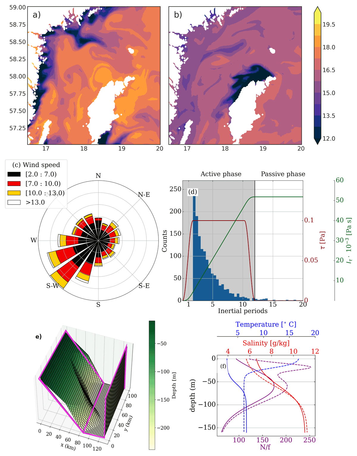
Figure 1
(a) Sea surface temperature (°C) from Copernicus Marine Service (CMEMS) sea state forecast (https://marine.copernicus.eu/, DOI: https://doi.org/10.48670/moi-00010, accessed 2023-07-18 14:38 UTC) during southwesterly winds in summer 2021 (upwelling on the Swedish coast, downwelling on the Gotland side). (b) As (a) but for northeasterly winds. (c) The wind intensity and direction 1996–2021, and (d) Histogram of the duration of southwesterly wind events from the Landsort station (https://www.smhi.se/data/meteorologi, accessed 2022-09-01) (left ordinate axis), and the applied wind forcing (right ordinate axis: wind stress, [Pa], red line, and the wind impulse, [Pa s], green line) in function of time (active phase is shaded); the time is normalized by the local inertial period. (e) Model bathymetry of the WGB (magenta: control simulation with a constant slope, shading: a sinusoidal variation (LANDSORT). (f) Summer (dashed) and winter (solid line) potential temperature and salinity profiles used to initialize the numerical model, and the Coriolis parameter scaled Brunt Väisäla frequency.
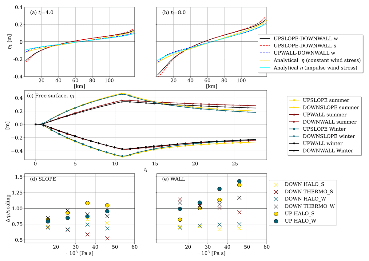
Figure 2
Top: Cross-shore profiles (inertial-period average) of the analytical and simulated alongshore averaged free surface at (a) and (b), for the winter simulation with a flat bottom (UPWALL-DOWNWALL) and summer and winter simulations with slope on one side (UPSLOPE-DOWNWALL). (c): Timeseries [inertial periods] of the alongshore-averaged free surface for different model experiments for slope () and wall () sides of the channel. (Bottom): Simulated interface (HALOcline and THERMOcline) displacements scaled with the analytical solution (Equation 27) in function of the wind impulse values at ti = 4, 6, 8, 10 for SLOPE (d) and WALL (e) marked by dots (crosses) for upwelling (downwelling) for winter. For wall side (e) we computed the interface depth at , while for slope side the interface depth is given by equation 3 using the closest location of the interface to .
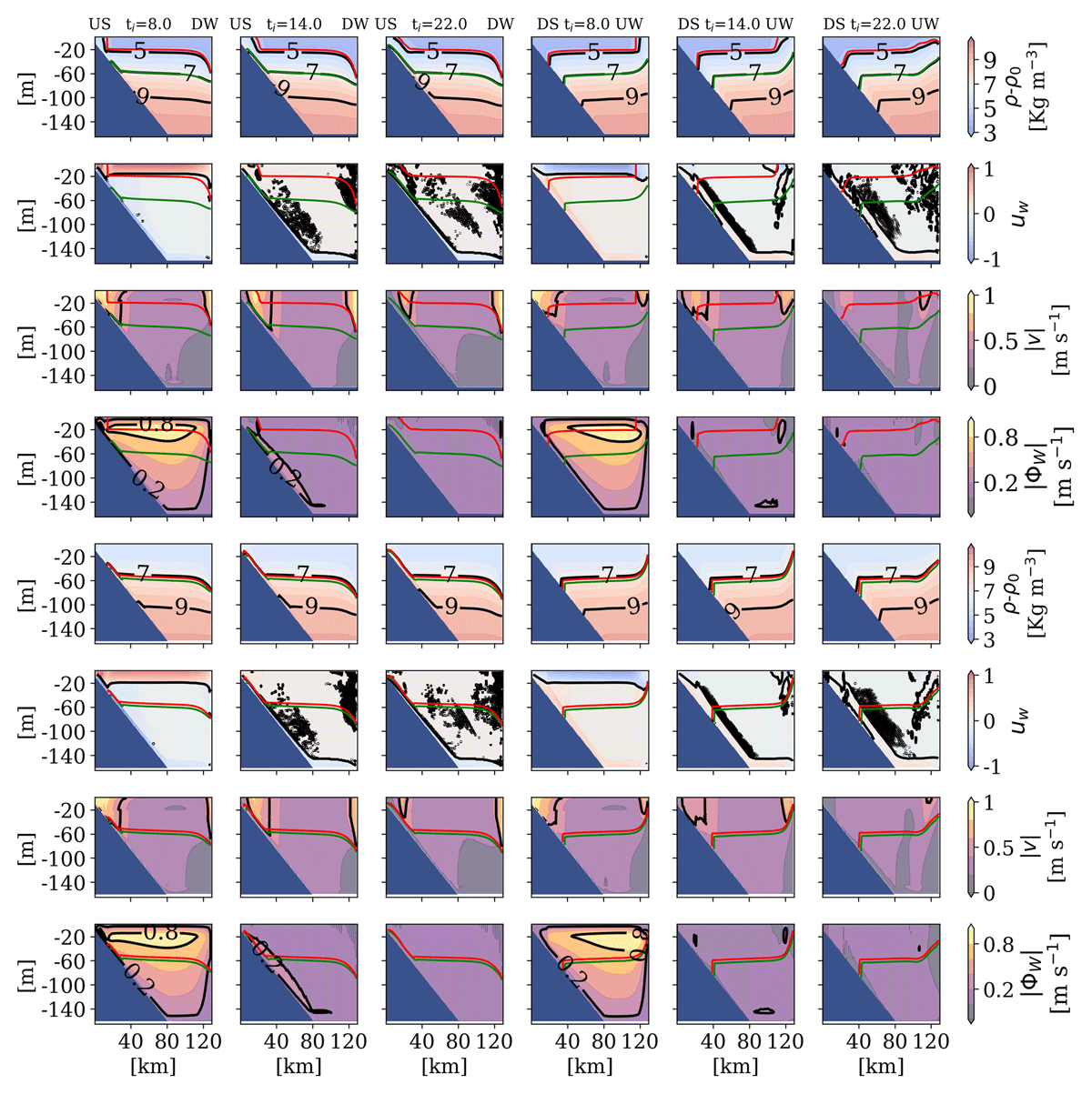
Figure 3
Cross-shore sections of density anomaly, Ekman transport-scaled cross-shore velocity uw, alongshore velocity v, and stream function at selected times [inertial periods], all averaged over one inertial period and in along-shore direction. The thermocline and halocline are marked with red and green lines, respectively. Positive wind stress (UPSLOPE-DOWNWALL) left panels, negative wind stress (DOWNSLOPE-UPWALL) right panels. Summer top, winter bottom.
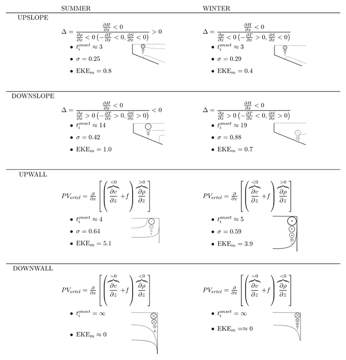
Figure 4
A schematic summary of the instability diagnostics for the different model configurations. EKE is given in 10–6 m2 s–2. Growth rate in day–1. See text for details.
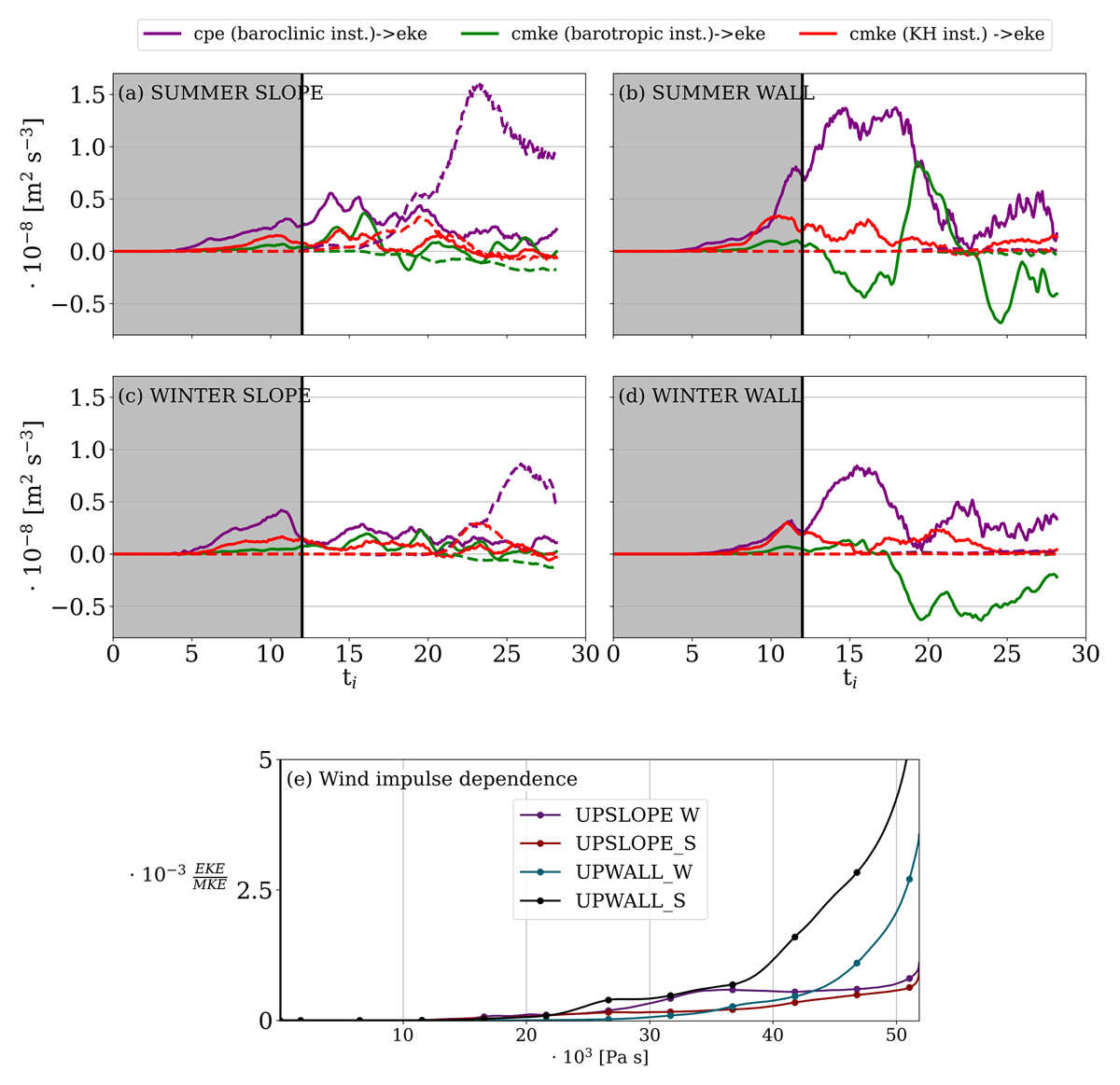
Figure 5
Energy conversion rates. Purple: CPE (PE to EKE, baroclinic instability), green: horizontal shear to EKE (barotropic instability), red: vertical shear to EKE (KH instability). (a and b): Summer SLOPE and summer WALL; (c and d): winter SLOPE and winter WALL. Solid and dashed lines show upwelling and downwelling, respectively. Shaded grey area marks the active phase. (e) Ratio of EKE to MKE (lower panel, c–d) on the wind impulse during the active phase. Dots mark inertial periods.
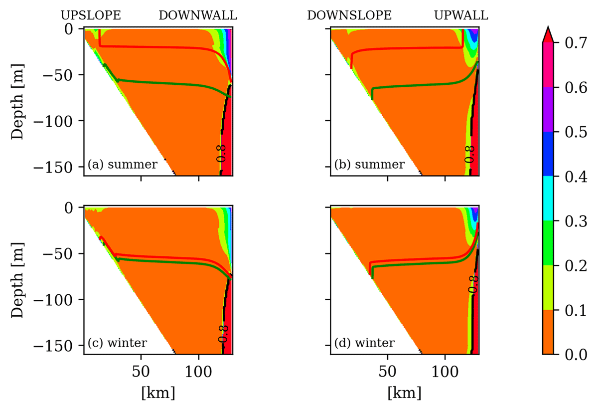
Figure 6
The ratio of the baroclinic component vbc (total subtracted the depth-average) to the total alongshore velocity v at ti = 8 for summer UPSLOPE-DOWNWALL and DOWNSLOPE-UPWALL (a–b) and winter UPSLOPE-DOWNWALL and DOWNSLOPE-UPWALL (c–d).
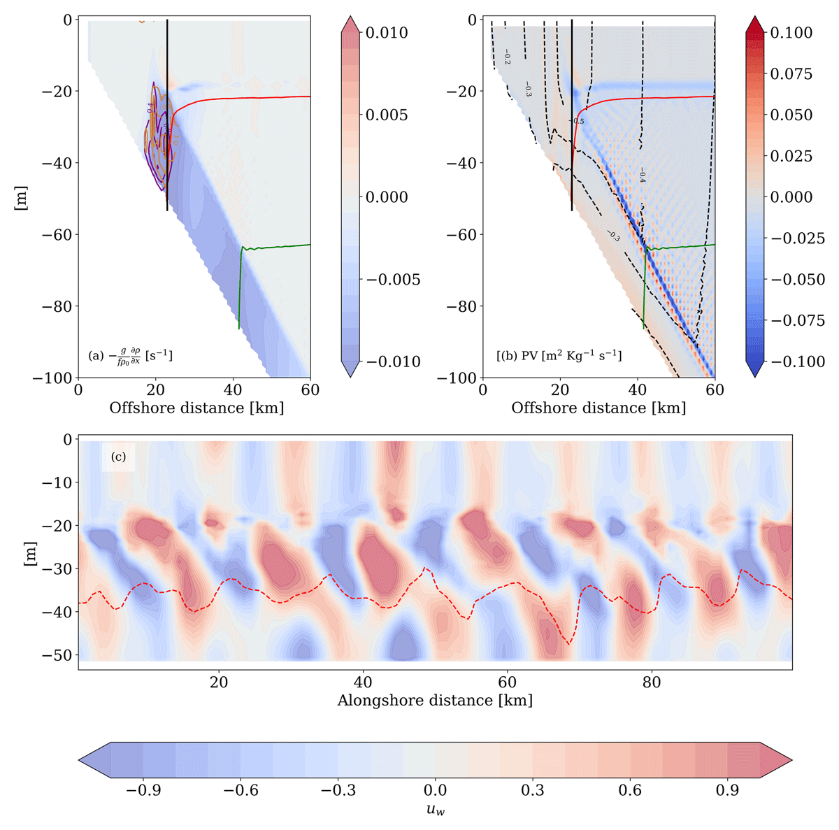
Figure 7
Instability diagnostics after the onset of instability (ti = 6) for UPSLOPE, summer. (a): Thermal wind overlapped with contours of cpe (purple lines) and cmke (green lines). Contour lines show the interval (0.4, 1.6) · 10–8, with every interval given by 0.4 · 10–8. Thermocline and halocline are given by the dashed red and green lines, respectively. The vertical solid black line marks the frontal jet location alongshore section in (c) is taken. (b) PV field contours of alongshore velocity (coastal jet; black lines). (c) Alongshore section of normalized cross-shore velocity uw at the frontal jet location (black solid line in (a)).
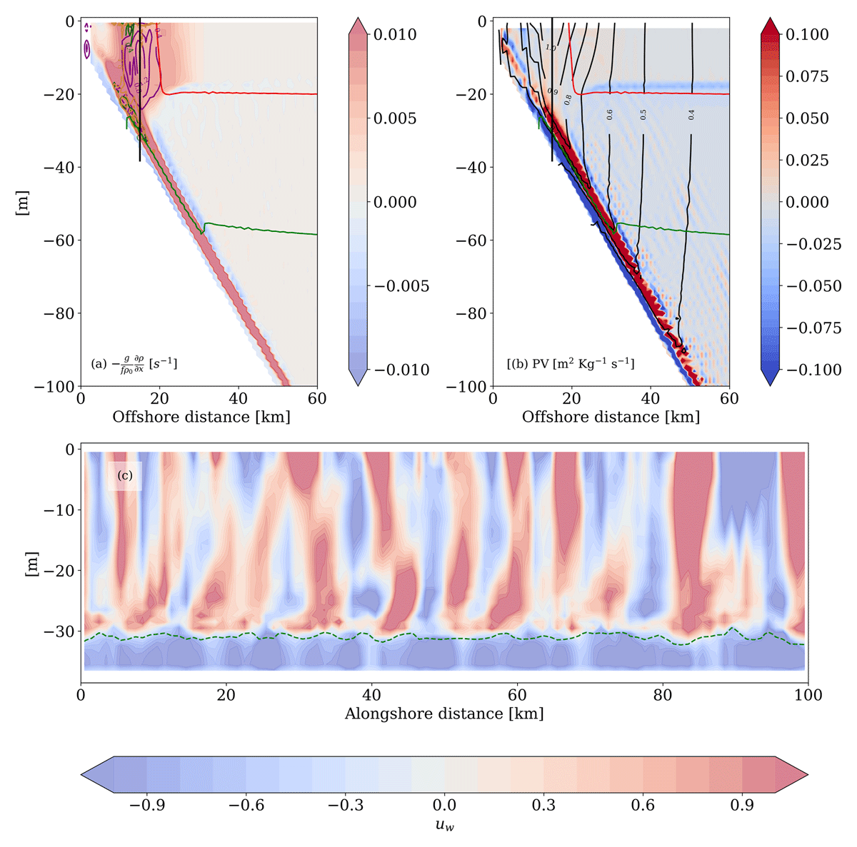
Figure 8
Same as Figure 7 but for DOWNSLOPE, summer, ti = 18.
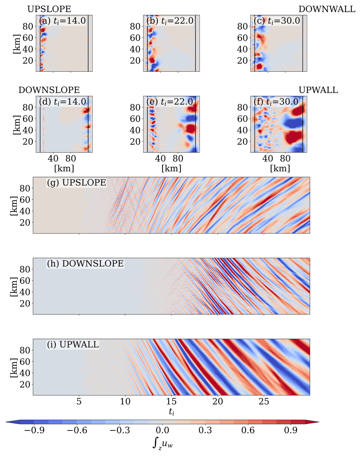
Figure 9
A top view of the depth-averaged cross-shore velocity field for positive wind stress (first row, a–c) and negative wind stress (second row, d–f) at ti = 14, 22, 30 in summer. Hovmöller diagrams for the depth averaged cross-shore velocity field at the location marked by the solid black line in panels above marking the location of the upwelling and downwelling front at the onset of instabilities: (g) DOWNSLOPE, (h) UPWALL, and (i) UPSLOPE.
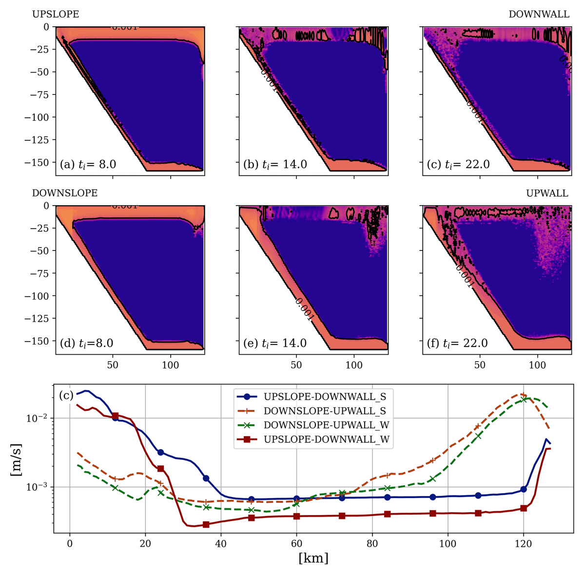
Figure 10
Alongshore averaged vertical viscosity coefficient from KPP scheme for UPSLOPE-DOWNWALL (upper panel, a–c) and for DOWNSLOPE-UPWALL (lower panel, d–f) at selected times ti = 8, 14, 22. Solid black line marks the contour of 10–3 m2 s–1. (g): Surface cross-shore eddy salinity fluxes averaged in the alongshore direction and between t = 10 t2 and 20 t2.
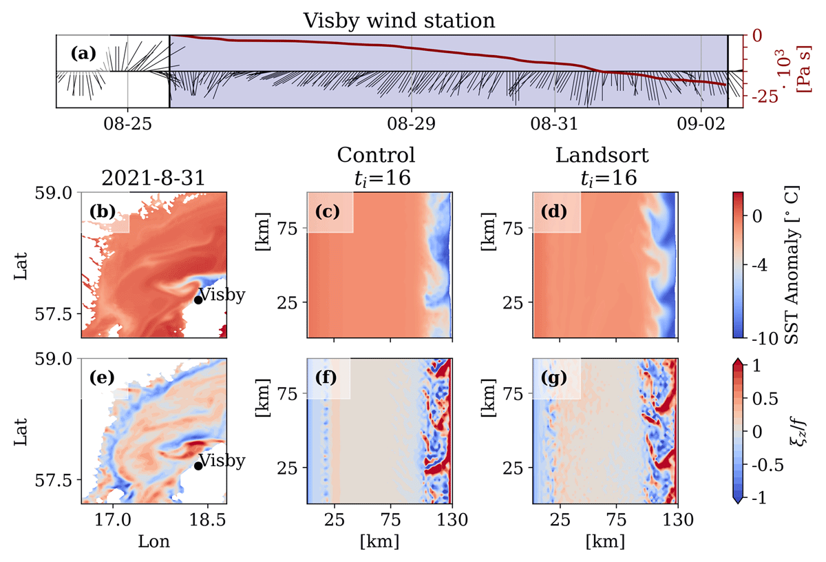
Figure 11
(a) Stickplot for wind speed and direction measured at the SMHI meteorological station in Visby during a northeasterly wind event in August 2021 (downloaded from http://opendata.smhi.se/apidocs/metobs/index.html, assessed on 29th April 2024, 14:58:24). On the right-axis, the alongshore wind impulse has been plotted (computed using equation 2 and by rotating the wind vector of 45° which is an approximate the coast direction and the N-S). Panels (b) and (e) show, respectively, the SST anomaly ([°C]) from the domain average on the 26th of August 2021 (prior to the upwelling event) and the vertical component of the relative vorticity at the surface ( derived from sea state forecast for the 2021-08-31 (https://marine.copernicus.eu/, DOI: https://doi.org/10.48670/moi-00010, accessed 2023-07-18 14:38 UTC). Panels (c) and (f) show the model anomaly surface potential temperature from the domain average at and the relative vorticity from the channel with uniform bathymetry (DOWNSLOPE-UPWALL summer), and the same field are plotted in (d) and (g) for simusoidally varying bathymetry (LANDSORT DOWNSLOPE-UPWALL summer) for .
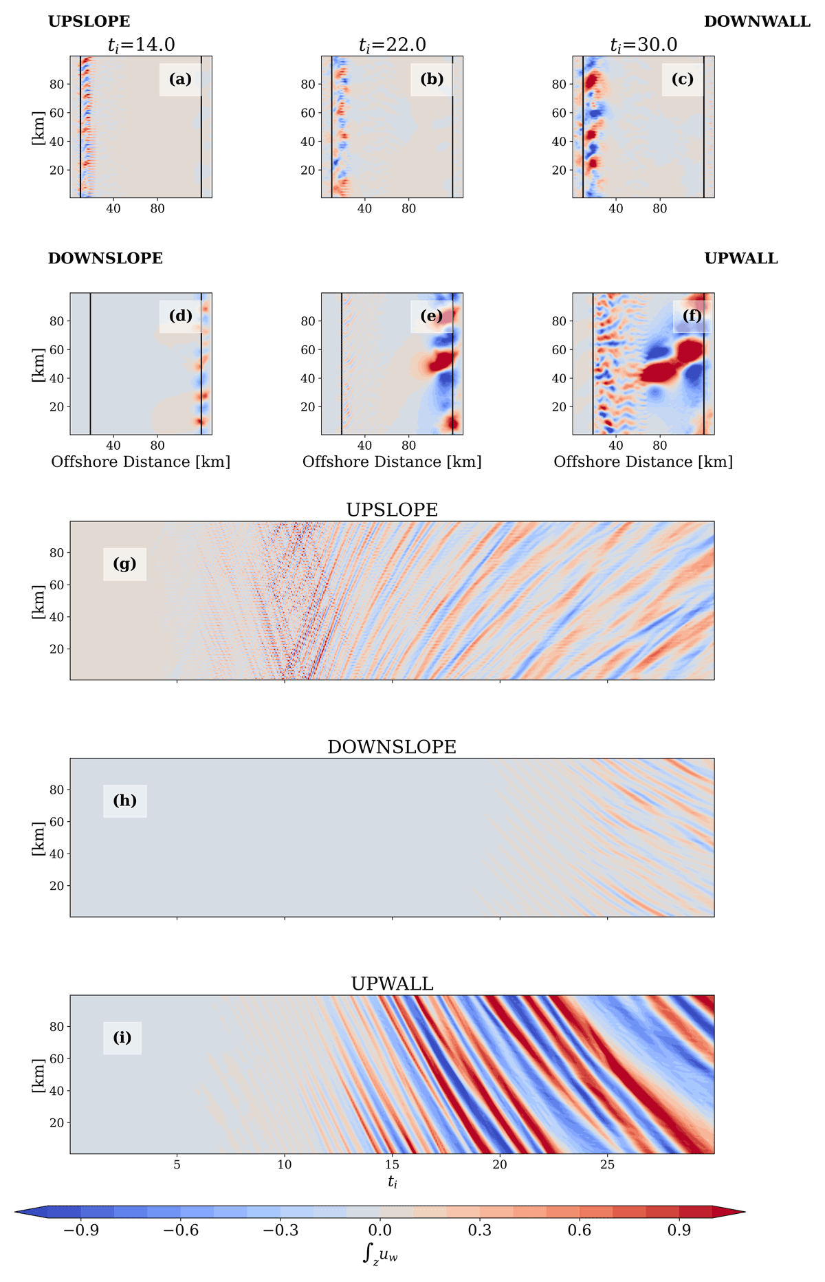
Figure A1
A top view of the depth averaged cross-shore velocity field for positive wind stress (first row, a–c) and negative wind stress (second row, d–f) at ti = 14, 22, 30 in winter. Hovmöller diagrams for the depth averaged cross-shore velocity field at the location marked by the solid black line in panels above marking the location of the upwelling and downwelling front at the onset of instabilities: (g) UPSLOPE, (h) DOWNSLOPE, and (i) UPWALL.
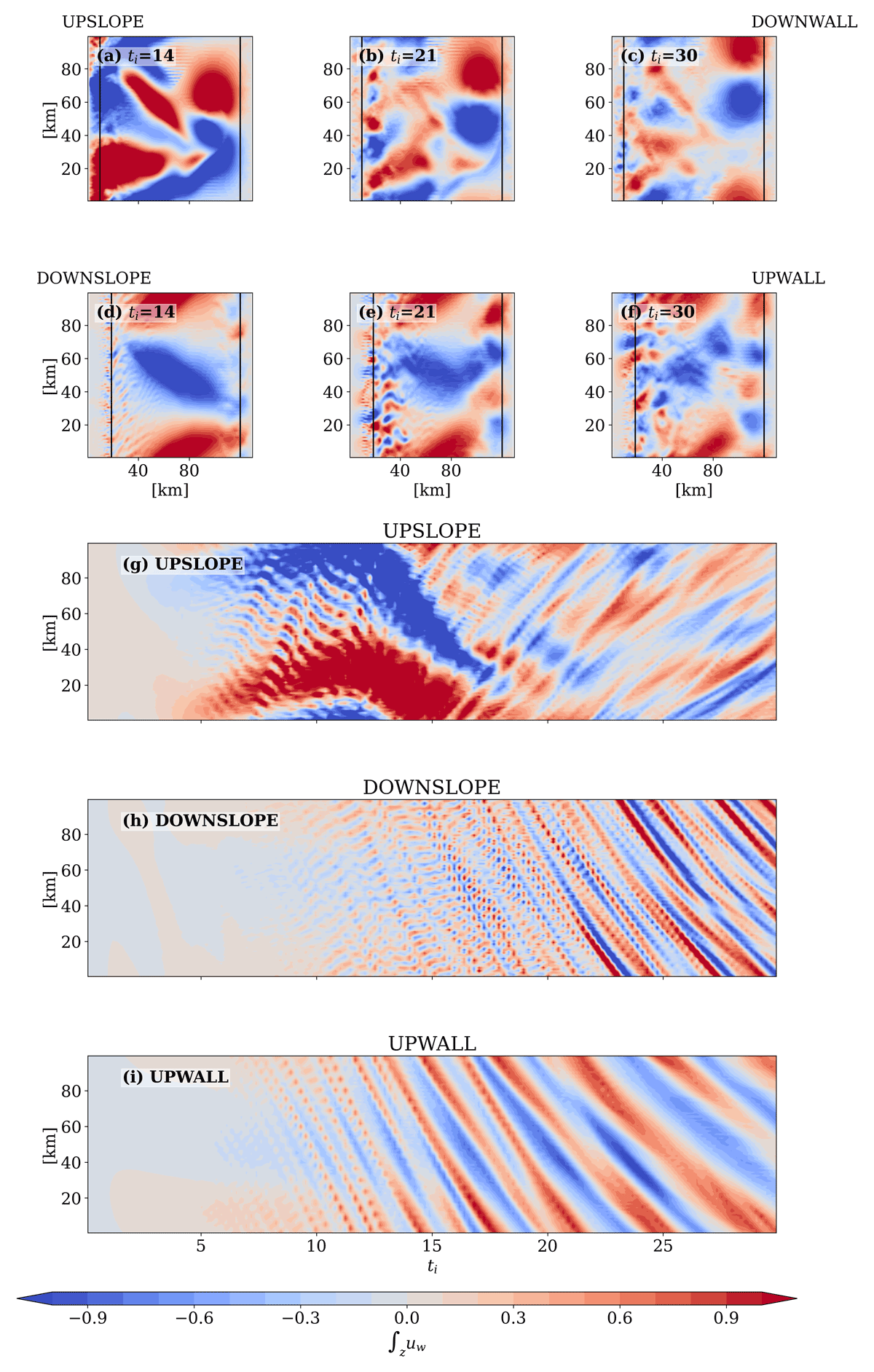
Figure A2
A top view of the depth-averaged cross-shore velocity field for positive wind stress (first row, a–c) and negative wind stress (second row, d–f) at ti = 14, 22, 30 for summer with alongshore varying bathymetry. Hovmöller diagrams for the depth-averaged cross-shore velocity field at the location marked by the solid black line in panels above marking the location of the upwelling and downwelling front at the onset of instabilities: (g) UPSLOPE, (h) DOWNSLOPE, and (i) UPWALL.
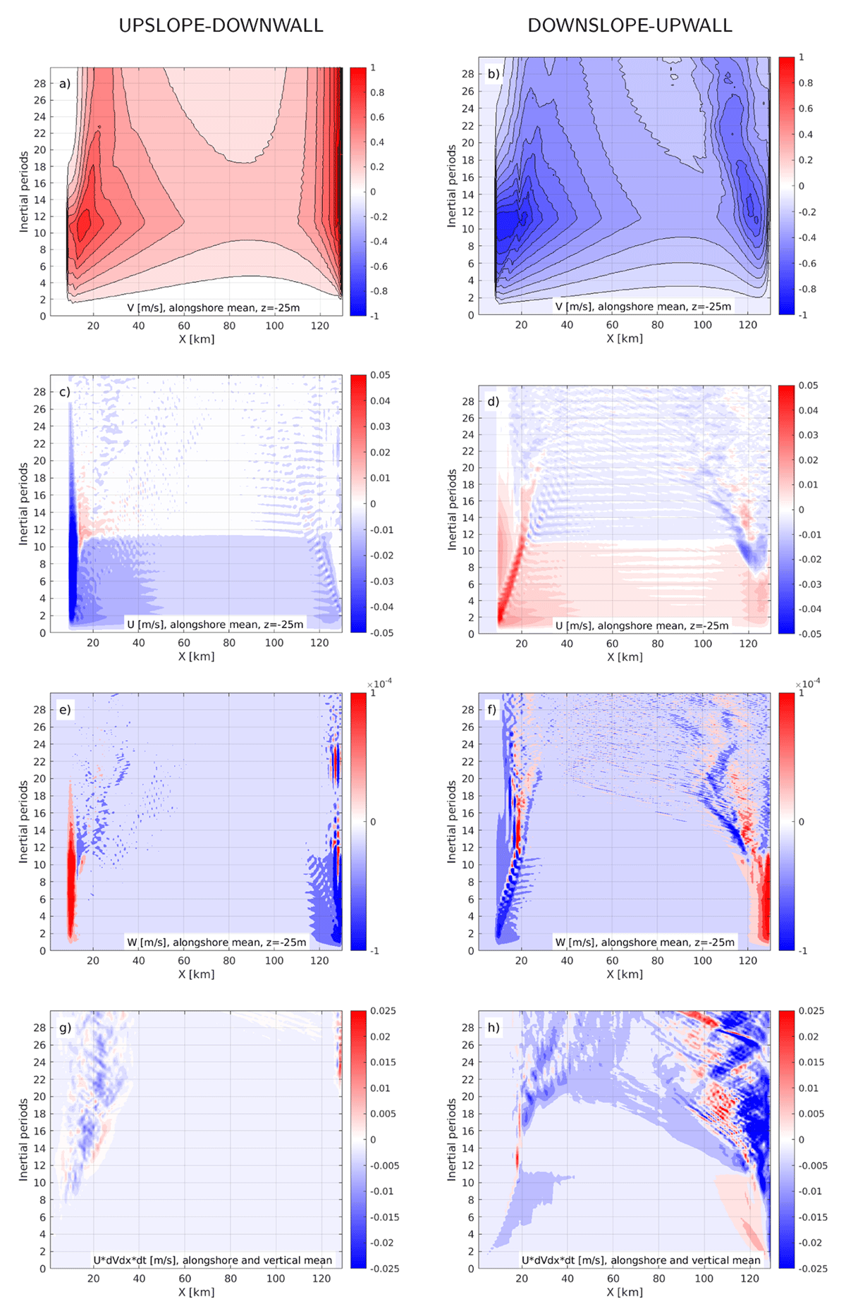
Figure A3
Three upper rows, from top to bottom: Hovmöller diagrams of alongshore averaged: alongshore velocity, cross-shore velocity and vertical velocity, respectively, at the 25 m depth. Bottom row: vertical- and alongshore average of alongshore velocity tendency due to cross-shore advection of alongshore velocity during one inertial period. Left: UPSLOPE-DOWNWALL; Right: DOWNSLOPE-UPWALL. All diagnostics are based on hourly averaged model output from summer simulations.