
Publisher’s Note: A correction article relating to this paper has been published and can be found at https://tellusjournal.org/articles/10.16993/tellus.4248.
1 Introduction
Upwelling in general refers to the vertical, displacement of deeper water towards the ocean’s surface. The opposite holds for downwelling. Upwelling (downwelling) is the result of divergence (convergence) of horizontal currents, and it is common in coastal regions. The most well-known are the Eastern Boundary Upwelling systems (hereafter, EBUs) on the Californian, Peruvian, Canary, and Benguela coasts; a permanent feature associated with trade winds raising the thermocline on the east side of the ocean basins, leading to a high surface concentrations of nutrients and high primary production (Chavez and Messié, 2009; García-Reyes et al., 2015). Wind-driven upwelling occurs also in other regions, e.g., along the East and West Greenland shelf (Håvik and Våge, 2018; Pacini and Pickart, 2023), on the Arctic shelves (Williams and Carmack, 2008) and locally in the Mediterranean Sea (Reul et al., 2005).
The Baltic Sea is a semi-enclosed shelf sea, where upwelling and downwelling are driven by several processes, including the transient alongshore winds, local wind curl, as well as the interaction of currents with topography (Fennel and Seifert, 1995; Lehmann and Myrberg, 2008; Myrberg and Andrejev, 2003), and are an important constituent of mesoscale dynamics, with substantial impacts on marine ecosystems and coastal services (Kullenberg, 1981; Lehmann and Myrberg, 2008). Specific to the Baltic Sea is the unique stratification given by a permanent halocline due to the basin-scale estuarine circulation driven primarily by freshwater runoff from land and intermittent deep saltwater inflows from the North Sea. The halocline is found at 60–80 m depth in the center of the basins, shoaling towards the coast. During summer, a shallow seasonal thermocline forms, typically at a depth of 20 m (Kullenberg, 1981; Lehmann and Myrberg, 2008). In several areas of the Baltic sea (for example, along the Swedish east and south-eastern coast, by the island of Gotland, in the Gulf of Finland and the Polish coast) the alongshore winds prevail and coastal upwelling is observed typically 25—40% of the time in the Sea Surface Temperature (SST) imagery, due to the lower temperature of the upwelled water (Lehmann et al., 2012; Sproson and Sahlèe, 2014). Observational studies focus on the upwelling of the thermocline; however, very few focus on the upwelling of the halocline and downwelling events, which are much harder to investigate through observations because of the transient nature of the phenomena and the absence of a clear SST signature on the surface.
The upwelling and downwelling response of the coastal ocean to transient wind forcing is dominated by (cross-shore) Ekman transport and the development of the (alongshore) coastal jets trapped to the coast within the distance determined by the Earth’s rotation and stratification (the so-called Rossby radius of deformation distance). In a stratified setting, the circulation can be decomposed into barotropic and baroclinic modes, directly related to the free-surface, and pycnocline, displacement(s), respectively (Csanady, 1982; Vallis, 2019). Adding a gentle sloping bottom and friction leads to displacement of the isopycnals over the bottom (Lentz and Chapman, 2004). The resulting horizontal density gradients and vertical shear of horizontal velocity (thermal wind) can lead to a cessation (buoyancy arrest) of the bottom Ekman transport (Brink and Lentz, 2010; Garrett et al., 1993).
In the Baltic Sea, the characteristic scale of the baroclinic disturbances, the baroclinic Rossby radius is in the order of 5 to 10 km (Fennel and Seifert, 1995) and the local inertial period (a time scale over which the Ekman flows develop) is about 14 h. Such small spatial scales are hardly resolved by the current operational models and regional ocean modeling studies using typically 1 or 2 nm horizontal spacing (Hordoir et al., 2019; Radtke et al., 2020). Modeling studies of a higher resolution exist, but these have focused on local vertical mixing or submesoscale processes (Chrysagi et al., 2021; Holtermann et al., 2014; Väli et al., 2017; Zhurbas et al., 2022). Some existing process studies that combined satellite observations and modeling (Gurova et al., 2013; Zhurbas et al., 2008) proposed that the upwelling and downwelling dynamics associated with transient wind events can be divided into two different stages: an active phase and a passive phase. In the active phase, when the alongshore wind is blowing, a coastal jet is developing. In the presence of alongshore bathymetric variations, satellite images show a meandering of the coastal jet, which has been explained in terms of the conservation of potential vorticity (Gurova et al., 2013).
In the passive phase, when the winds weaken and veer, the strong horizontal temperature gradients developed during upwelling can persist for several days. Coastal jets were found to become baroclinically unstable leading to the formation of an eddy field and high cross-shore eddy diffusivity values, implying increased cross-shore transport of heat and upwelled nutrients (Zhurbas et al., 2008), before the next alongshore transient wind event starts resetting the system.
Idealized simulations in a circular basin with variable f show that both upwelling and downwelling coastal jet undergo baroclinic instability (Zhurbas et al., 2006). High-resolution idealized simulations in response to weak transient winds reveal that baroclinic instability is the main mechanism determining the decay of the coastal jet on a sloping bottom relying on the analysis of energy diagnostics (Brink, 2016; Brink and Seo, 2016).
Upwelling and downwelling events have numerous potential implications for the Baltic Sea marine ecosystem and coastal services. The properties of the atmospheric boundary layer and the flux of carbon dioxide through the air-sea interface may be affected by the colder up-welled waters (Norman et al., 2013; Sproson and Sahlèe, 2014).
Coastal upwelling has important consequences for primary production, which have not yet been fully understood. For example, downwelling and upwelling conditions during summer appear to have a net negative effect on cyanobacteria blooms. One reason for this is that the most abundant cyanobacteria have a high temperature optimum and their growth is inhibited due to the colder and saltier up-welled water, further due to strong mixing associated with both upwelling and downwelling events (Dabuleviciene et al., 2020; Kanoshina et al., 2003; I. Lips and Lips, 2008; Olofsson et al., 2020, 2019). On the other hand, the coastal upwelling may be one of the drivers triggering summer cyanobacterial blooms by supplying the phosphates to the surface layer in the summer after the spring bloom has depleted them. (Larsson et al., 2001; Zhurbas et al., 2008). Studying downwelling and upwelling as the mechanism modulating algae bloom occurrence has indirect importance for the marine food web (A. M. L. Karlson et al., 2015; B. Karlson et al., 2021) and the local tourism industry, as algae blooms reduce water quality and make coastal waters unattractive for recreation (Wasmund, 2002).
In this study, we focus on the region of the Baltic Sea between the Swedish east coast and the Gotland Island (Western Baltic Proper, or Western Gotland Basin, WGB), featuring prevailing southwesterly winds of a few days duration favorable to upwelling on the Swedish coast [about 30% time, (Lehmann and Myrberg, 2008), see also Figure 1c–d]. Because of the channel-like bathymetric setting, the upwelling and downwelling events develop concurrently on the two sides of the basin (Figure 1a–b). None of the previous studies of upwelling, either in a general setting or in the Baltic Sea, considered a geometry specific to WGB (Figure 1e) in a systematic manner or provided results on the lifecycle and instability processes occurring on both sides of the WGB. The WGB is further unique for the bottom bathymetry which is very different on the two sides of the 100–150 km wide channel: the western (mainland) side descends to the sea with a gentle slope, while the slope of the eastern (Gotland) side is dramatically steep. The center of the channel is characterized by the presence of alongshore bathymetric variations culminating into the deepest point of the Baltic Sea (459 m).
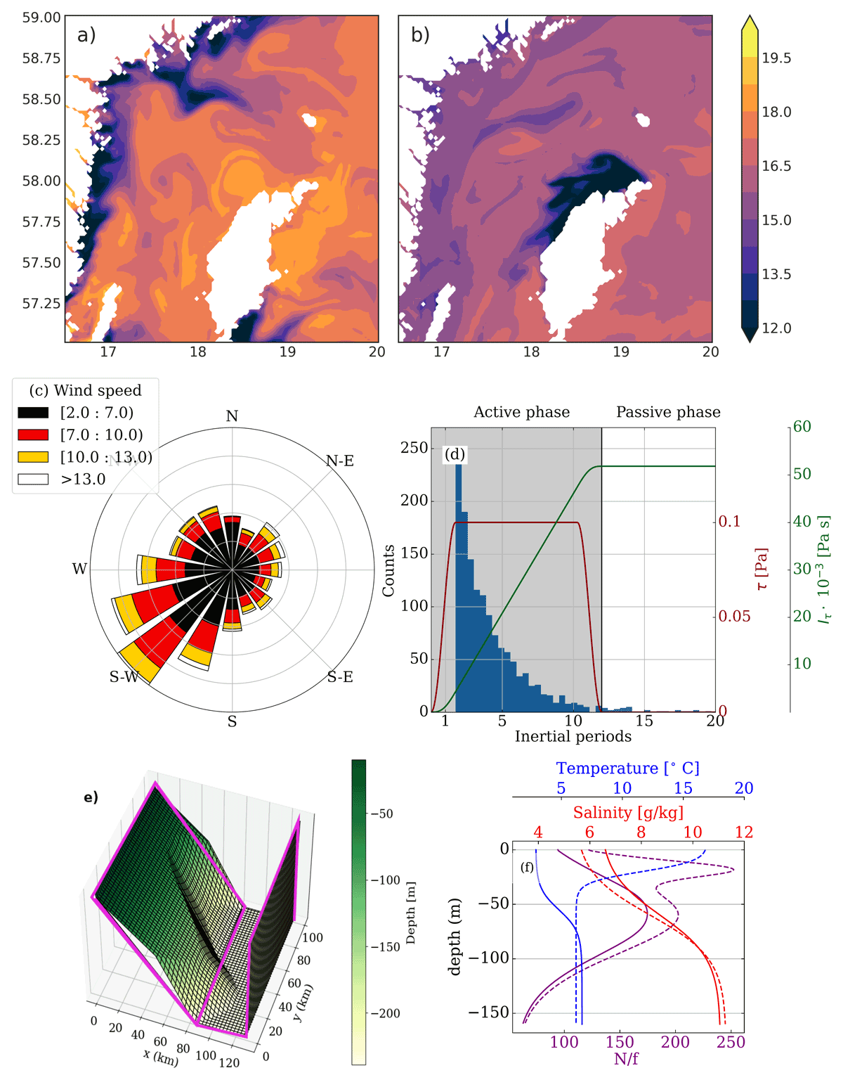
Figure 1
(a) Sea surface temperature (°C) from Copernicus Marine Service (CMEMS) sea state forecast (https://marine.copernicus.eu/, DOI: https://doi.org/10.48670/moi-00010, accessed 2023-07-18 14:38 UTC) during southwesterly winds in summer 2021 (upwelling on the Swedish coast, downwelling on the Gotland side). (b) As (a) but for northeasterly winds. (c) The wind intensity and direction 1996–2021, and (d) Histogram of the duration of southwesterly wind events from the Landsort station (https://www.smhi.se/data/meteorologi, accessed 2022-09-01) (left ordinate axis), and the applied wind forcing (right ordinate axis: wind stress, [Pa], red line, and the wind impulse, [Pa s], green line) in function of time (active phase is shaded); the time is normalized by the local inertial period. (e) Model bathymetry of the WGB (magenta: control simulation with a constant slope, shading: a sinusoidal variation (LANDSORT). (f) Summer (dashed) and winter (solid line) potential temperature and salinity profiles used to initialize the numerical model, and the Coriolis parameter scaled Brunt Väisäla frequency.
The WGB coastal zone features a high-density population, a marine industry, and intense summer touristic activity around the Stockholm Archipelago and on Gotland, all of which are to some degree directly affected by water temperature changes and mixing, induced by upwelling and downwelling, or indirectly, through the implications for algae blooms and the marine ecosystem. A conspicuous example is the desalination plants at Kvarnåkershamn and Herrvik, located on the west and east Gotland coast, respectively, to produce drinking water from sea water, making an important supplier to the island’s water resources. The desalination process uses water pumped from 6–12 m depth and operates in two modes: summer and winter. Sudden temperature changes associated with the upwelling and downwelling events, as well as the organic algal accumulations associated with them, disturb the desalination process [Region Gotland, pers. comm.. An increased understanding of the upwelling signal along the Gotland coast will support the forecasting for the desalination process on the island, which is the goal of the ALGOTL project.
In this work, we study the development of coastal upwelling and downwelling responses to typical transient winds in an idealized model configuration representative of the WGB channel-like geometry and stratification. We study the development and relaxation of coastal jets and associated instability processes building upon previous modeling studies of upwelling and downwelling (Brink, 2016; Durski and Allen, 2005; Zhurbas et al., 2008), complemented by theoretical considerations based on Csanady (1982) and Stipa (2004) and analysis of instability conditions and scales. We find the characteristic WGB geometry (a channel of finite width with a sloping bottom on one side) combined with the Baltic Sea stratification and typical wind field introduces new aspects into the lifecycle of wind-driven flows, compared to the previous literature, in particular an asymmetric response on the two sides of the channel in terms of the stability conditions the instability growth rates, and length scales varying dependent on the presence of the sloping boundary, wind direction, and seasonal stratification. We also assess implications for horizontal and vertical transport processes in the region.
The forthcoming sections of this paper are organized as: Section 2 introducing the numerical model and the diagnostics; followed by Section 3 where we present and discuss the results from our model simulations complemented by theoretical considerations; summarized by conclusions in section 4.
2 Methods
2.1 Basic model configuration
We use the Massachusetts Institute of Technology general circulation model (MITgcm; http://mitgcm.org), an open-source FORTRAN solver for Primitive Equations (the Boussinesq form of the Navier–Stokes equations). MITgcm employs a finite-volume discretization rendered on a horizontal Arakawa C-grid, with vertical z-levels employing partial cells (Adcroft et al., 2004; Marshall et al., 1997). The MITgcm has been used previously for idealized regional circulation studies including upwelling (Dawe and Allen, 2010; Howatt and Allen, 2013; Thomsen et al., 2021).
In our study, we consider a high-resolution, idealized, hydrostatic setup of the WGB. A Cartesian coordinate system () has horizontal axes aligned with the cross-shore direction (x; width ) and the alongshore direction (y; width ). The three-dimensional velocity vector in this coordinate system is . Periodic boundary conditions are applied in the alongshore direction, and closed boundaries in the cross-shore direction at the Swedish east coast and Gotland (Figure 1e). On these scales, the latitudinal variation of the Coriolis parameter is negligible and we apply a f-plane for 58° N (), corresponding to one inertial period of .
Our idealized model configuration is focused on the dynamics of sub-inertial motions (inertial waves are merely transient phenomena given the applied forcing and wind waves are not resolved here). We apply a fully implicit time stepping (https://mitgcm.readthedocs.io/en/latest/algorithm/crank-nicol.html), thus neglecting the time variations of free surface when computing the horizontal transports in the continuity equation and in tracer and momentum advection terms. This method is unconditionally stable and avoids computational effort related to the implementation of the non-linear free-surface formulation, but it damps the fast gravity waves. The horizontal resolution is and the vertical resolution is . In the horizontal, the viscosity and diffusivity are parameterized with a Laplacian operator with a viscosity of 10–5 m2 s–1 and temperature and salinity diffusivities are kept at lowest possible, i.e., default molecular diffusivities of 10–7 m2 s–1 and 10–9 m2 s–1, respectively, to avoid excessive smoothing of fronts (so in practice the horizontal diffusivities are negligibly small). In the vertical, a non-local K-Profile Parameterization (KPP) scheme (Large et al., 1994) is used to parameterize vertical mixing: the background value of vertical viscosity and tracer diffusivity (both equal to 10–6 m2 s–1) are modified in the surface boundary layer by employing the Monin-Obukhov similarity theory, accounting for non-locality of the turbulent fluxes, which depend on the boundary layer depth and surface fluxes, in addition to local properties and gradients. In the interior, the vertical viscosity and diffusivity depend on the velocity shear and stratification to represent shear instability and internal wave breaking. The vertical dissipation is thus a function of the system state and will vary between the configurations. The use of KPP circumvents the necessity of setting high values of vertical viscosity and diffusivity coefficients everywhere in the domain to ensure the numerical stability in the more vertically diffusive boundary layers. It also allows us to quantify vertical turbulent transport associated with the resolved dynamics (see Figure 10a–f and section 3e.).
The bottom stress is given by the linear friction law , where ub and vb are horizontal bottom velocity components and the bottom drag coefficient is r = 10–4 m s–1 as used in Brink (2016), and with as the model reference water density. Heat fluxes are set to zero.
2.2 Wind forcing
The model is forced with an alongshore wind stress variable in time following:
This corresponds to a single wind pulse of the duration of 12 inertial periods where the period of maximum wind amplitude, , is equal to 8.45 inertial periods (five days), which is approximately the center of distribution of upwelling event duration (Figure 1d) and long enough for the instabilities to develop. The wind stress is initialized with (1 day), before reaching the constant amplitude N m2 (negative for upwelling on the Swedish east coast side and for downwelling on the Gotland side), corresponding to gentle breeze conditions on the Beaufort scale (7–10 m s–1), typical to WGB (Figure 1c).
The wind is spatially uniform, which is a reasonable assumption based on wind observations in WGB (not shown), see also Lehmann and Myrberg (2008). The shape of the wind stress function (for positive values) is superimposed on Figure 1d. The wind impulse is defined as:
and quantifies the input of the wind momentum due to a given wind stress and duration of the wind event. The total time for model experiments and analysis is month = 28 days, i.e., longer than the transient wind time scale in the region (Figure 1c–d).
2.3 Bathymetry
The bathymetry setting is a channel with a sloping bottom on the west (Swedish coast) side and a vertical wall on the eastern (Gotland) side (Figure 1e):
where is the basin depth and the slope parameter α is equal to the average slope south of the Landsort Deep, . The bending point of the slope is at where the bottom becomes flat until the Gotland coast at .
Two model runs using this bathymetric setup with alongshore winds of opposite directions result in four flow regimes: UPSLOPE (upwelling on the slope side) with DOWNWALL (downwelling on the wall side), and DOWNSLOPE (downwelling on the slope side) with UPWALL (upwelling on the wall side). The regimes are demarcated by the slope bending point at .
We complement our study with the simulation LANDSORT, including a sinusoidal alongshore bathymetric variation (alongshore wavenumber ) mimicking the basin-scale feature in the WGB (a trough at the Landsort Deep). We do not consider the deepest part of the Landsort Deep below –160 m, but since the density gradients are very weak below –100 m (Figure 1f and Section 2.4), we assume that it does not impact the dynamics of the coastal upwelling at the basin scale. We also run a simulation with no slope vertical walls on both sides) to compare with the analytical two-layer model. We evaluated the sensitivity to horizontal resolution by running a higher resolution simulation () and also to the bottom drag formulation (by running a simulation with quadratic bottom drag). Both sensitivity runs have been initialized with winter stratification.
2.4 Stratification
The simulations are initialized with continuous stratification profiles representative of summer (August) and winter (March) conditions taken from the Copernicus Marine Service (CMEMS) reanalysis and forecast [https://data.marine.copernicus.eu/product/BALTICSEA_ANALYSISFORECAST_PHY_003_006/. Product DOI: https://doi.org/10.48670/moi-00010. The reanalysis profiles were averaged over a transect parallel to the coast and idealized by the following analytical expressions:
where S0 and T0 are, respectively, the salinity and temperature at the surface, while S1 and T1 represent, respectively, the bottom values and z0 and z1 are fitting parameters. The idealized profiles smooth over noise and neglect the deep temperature minimum in the summer profiles, which is of minor importance for the dynamical processes studied here, but it might be important for more realistic studies of WGB circulation in the future. The resulting profiles used to initialize the model are shown in Figure 1f. During the month of August, the summer thermocline is well developed at 20 m with surface waters up to 10°C warmer than deeper layers. Example upwelling and downwelling expressions on the summer SST field are shown in Figure 1a–b. During winter (March), the upper thermocline is reversed (colder water at the surface) and weaker (3°C difference), with a more distinct mixed layer.
The salinity and halocline do not show a pronounced seasonal cycle, as it is set by the estuarine circulation in the Baltic Sea dominated by interannual variability (Kullenberg, 1981; Lehmann et al., 2022). Figure 1f includes the corresponding profiles of the squared buoyancy (Brunt–Väisäla) frequency computed from the potential density referenced to the surface:
This displays one, and then two, distinct pycnoclines in summer and winter, respectively: the summer thermocline forms a distinct summer pycnocline above the main one, strenghtening the stratification; while the winter thermocline is located only slightly above the main pycnocline (halocline) and has a weakening effect on the stratification.
2.5 Scales of motion
For (flat bottom), the barotropic Rossby radius of deformation is (the gravity wave speed ). We can estimate the baroclinic Rossby radius of deformation, Rbc, from the two-layer model which is representative for the Baltic winter stratification:
where , and are the thickness and density of the layer above a pycnocline, and are the thickness and density of the layer below, so that . The value of Rbc given by equation 6 is comparable with the estimate of the baroclinic Rossby radius of deformation using the first eigenvalue of the vertical normal mode decomposition Fennel et al. (1991) and Zhurbas et al. (2006), which yields about 8 km for summer and 7 km for winter stratification. Throughout the manuscript, we only use Rbc as an estimate of the baroclinic Rossby radius. The baroclinic gravity wave speed estimate yields .
A non-dimensional number quantifying the effects of sloping topography and stratification is the topographic Burger number (Lentz and Chapman, 2004):
This number gives an estimate of the proportion of the volume transport confined to the bottom boundary layer (Jacox and Edwards, 2011): lower values indicate that the surface wind stress is compensated by the bottom stress, indicating strong cross-shore volume transport in the boundary layer. As the Burger number increases, the contribution from cross-shelf momentum divergences increases, together with the volume transport in the interior. In our configuration, given the varying stratification, the Burger number can be estimated to be in the interval for all simulations.
To interpret the results related to sub-inertial dynamics, the time is non-dimensionalized by the local inertial period:
The cross-shelf stream function is defined in such a way that positive values describe an anti-clockwise overturning cell in an x–z plane and is non-dimensionalized as:
together with the cross-shore velocity field uw:
where
is an estimate of the Ekman layer thickness calculated using the value for the vertical viscosity computed by KPP scheme in the surface or bottom layer. The non-dimensionalization of Equations 9–11 sets the reference for the interpretation of the results.
2.6 Energy and instability diagnostics
We use a set of diagnostics introduced by Orlanski and Cox (1973) and applied in Brink (2016) and Durski and Allen (2005). Starting by defining the alongshore mean for a generic three-dimensional quantity :
together with its fluctuation from the alongshore mean:
with the spatially uniform wind forcing and bathymetry defined in equation 3, the deviations from the alongshore mean diagnose the instability processes in the domain.
The kinetic energy associated with the alongshore mean flow (MKE) is:
and the eddy kinetic energy (or EKE) associated with its perturbation:
where () are set respectively to (0,80) km and (80,130) km for the flow regimes on the sloping (subscript 1) and wall (subscript 2) sides separated by the slope bending point, and A is the averaging area.
Applying the averaging procedure to the equations of motion, the time variation of the total (summed slope- and wall side contributions defined in equation 15) eddy kinetic energy can be expressed as (Orlanski and Cox, 1973):
Note also the cross-shelf energy flux in equation 16 must sum to zero. In the following, we focus on the energy conversion terms diagnosing instability. The conversion from potential to eddy kinetic energy (cpe) can be split to the sum of a term associated with geostrophic adjustment and another term associated with baroclinic instability:
The conversion from mean to eddy kinetic energy (cmke) can be split into the component associated with the horizontal shear and another component with the vertical shear. The former is related to barotropic instability, while the latter is related to Kelvin-Helmholtz instability:
The onset of instability is estimated as the time when either of the energy diagnostics becomes different from zero. We estimate the instability growth rate as:
where and are the time at which the EKE reaches half and one-quarter of its maximum (Brink, 2016). To gauge the mechanism allowing for the development of instabilities we complement our analysis with Ertel potential vorticity (PV) computed following Morel et al. (2019), their Equations 11–14:
where the relative vorticity:
and ; together with thermal wind and the associated horizontal density gradients.
3 Results and discussion
This section begins with a linear analytical solution for coastal jets in a channel basin without slope displaying salient features recovered in the numerical solutions, of which are discussed in further detail hereafter.
3.1 Analytical linear solution for coastal jets in a channel basin
To determine the major features of upwelling and downwelling in an idealized WGB channel, and to assess our numerical model simulations, we derive an analytical solution for two-layer inviscid linear Ekman flow in a channel following the approach of Csanady (1982) however, we apply a wall boundary on both sides of the domain instead of the semi-infinite (open ocean) boundary used in previous works. For an alongshore wind forcing switched at and staying constant thereafter, the solution valid for small displacements of the interfaces (the free surface and the pycnocline) gives the following expression for a non-oscillatory component of the free surface displacement that grows linearly in time and is negative (positive) at the coast for upwelling (downwelling):
The constants and are given by the:
The free surface displacement is decomposed into barotropic () and baroclinic () modes, with the latter giving a minor contribution to the free surface displacement. The integrated velocity in the upper layer is also decomposed into barotropic and baroclinic components (Csanady, 1982):
The amplitude of the interface displacement is also evolving linearly in time and the transport in the lower layer yields (positive for upwelling):
Note that cross-shore velocities are independent of time while alongshore velocities grow linearly in time and form coastal jets trapped to the coast within a distance determined by channel width Lx and stratification (, Equations 22–24), anti-symmetrically about the zero-crossing point of the hyperbolical function at approximately . The closed boundary conditions in the cross-shore directions within the channel require that ( at and ).
The above solution describes wind-driven flows in a two-layer channel with vertical walls (no slope, no friction effects) and is valid only for the time period before the interface displacements become large and nonlinear effects kick in. Analyzing differences between the analytical and numerical solutions allows us to assess the role of friction, slope, the seasonal variations in stratification and the nonlinear effects. Figure 2a–b show the free surface profile (related to the barotropic component of the coastal jet) in the winter simulation with walls on both sides as well as simulations with slope on one side (scaled by the difference in domain volumes) for summer (three-layer-like continuous) and winter (two-layer-like continuous) stratification, and for both, constant wind stress and a wind impulse stress (see Equation 1) applied in our numerical simulations (only the simulations with negative wind direction are shown).
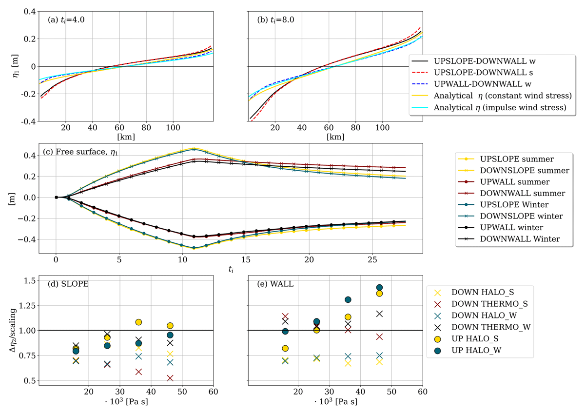
Figure 2
Top: Cross-shore profiles (inertial-period average) of the analytical and simulated alongshore averaged free surface at (a) and (b), for the winter simulation with a flat bottom (UPWALL-DOWNWALL) and summer and winter simulations with slope on one side (UPSLOPE-DOWNWALL). (c): Timeseries [inertial periods] of the alongshore-averaged free surface for different model experiments for slope () and wall () sides of the channel. (Bottom): Simulated interface (HALOcline and THERMOcline) displacements scaled with the analytical solution (Equation 27) in function of the wind impulse values at ti = 4, 6, 8, 10 for SLOPE (d) and WALL (e) marked by dots (crosses) for upwelling (downwelling) for winter. For wall side (e) we computed the interface depth at , while for slope side the interface depth is given by equation 3 using the closest location of the interface to .
After a spinup of ti = 2, the free surface displacement in the winter wall-wall simulation follows the analytical solution nearly exactly during the active phase. The free surface displacement over the slope is larger by 50% compared to the wall side due to higher wind momentum transfer per unit depth and the zero crossing is moved by about 10 km towards the coast. As a result, the free surface gradient () is stronger on the slope side, leading to a stronger barotropic flow there (over the course of time, this excess of momentum transfer in simulations is redistributed in the domain to the wall side leading to a stronger flow than the analytical solution there as well).
Notably, the distance over which the coastal flows on both sides are confined to the coast is set primarily by the channel geometry (width and slope). Seasonal variations of stratification (resulting in only a small range of Rbc) have a negligible effect. On the wall side, the free surface displacement continues to grow linearly and anti-symmetrically for upwelling and downwelling reaching ~0.45 m at the end of the active phase in agreement with the analytical solution. On the slope side, it grows at a higher rate albeit in a sub-linear manner (slower in the beginning as it takes time to develop boundary layer circulation). A slow relaxation during the passive phase follows reducing the displacement by half after one month.
Because the simulated stratification is continuous and the definition of interfaces is thus arbitrary, we can only gauge a qualitative comparison with the analytical solution. The model thermocline (halocline) are defined as isotherms (isohalines) corresponding to the maximum vertical gradient of the initial temperature (salinity) profiles in Figure 1f. Their maximum displacements also grow linearly in time during the active phase in agreement with the two-layer theory (Equation 27) but only for a period before the outcrop of the summer thermocline for UPWALL-S and UPSLOPE-S (about ti = 4) preceding onset of the instability (see Section 3.3), and similarly before shoaling of the winter thermocline for UPWALL-W after ti = 10 (for UPSLOPE-W the winter thermocline stays below 10 m, not shown). To further quantify this, we plot the simulated interface displacements scaled with the analytical solution (Equation 27) in function of the wind impulse in Figure 2d–e. The agreement between the simulated interface displacements and the analytical solution (derived for a channel with two walls) is within ±50% and is, as expected, better on the wall side (half of the values fall within ±25%). On the slope side, the analytical solution tends to be underestimated, in particular for the summer halocline. Note that there is uncertainty related to the definition of the interface and continuous stratification in the simulations). For stronger wind impulses, the interface outcrops and instabilities make the interface displacements deviate from analytical solution for the UPWALL (by a factor of >1.25) where instabilities set on early during the active phase (see Section 3.3). The scaling with wind impulse suggests that although neither the winter thermocline nor halocline outcrop in simulations presented here, they would do so if the wind impulse (strength and/or duration) would be increased by about 15% and 30% respectively (these however correspond to quite rare wind conditions in the WGB, see Figure 1c).
3.2 Coastal jets in a channel basin
The evolution of the flow for positive wind stress (UPSLOPE/DOWNWALL) and negative wind stress (DOWNSLOPE/UPWALL), summer and winter, is further analyzed in Figure 3 for selected time instances ti = 8, 14, 22. The first time instance is representative of the flow when the coastal jet is fully developed in the active phase, the second and the third represent, respectively, early and late stages of the passive phase when instabilities are present. Shown are the density anomaly, cross-shore, alongshore velocity, and streamfunction.
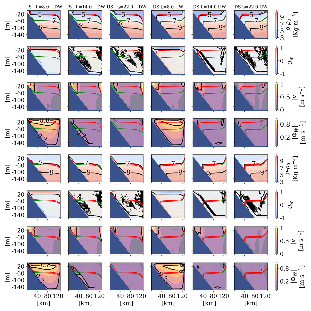
Figure 3
Cross-shore sections of density anomaly, Ekman transport-scaled cross-shore velocity uw, alongshore velocity v, and stream function at selected times [inertial periods], all averaged over one inertial period and in along-shore direction. The thermocline and halocline are marked with red and green lines, respectively. Positive wind stress (UPSLOPE-DOWNWALL) left panels, negative wind stress (DOWNSLOPE-UPWALL) right panels. Summer top, winter bottom.
In the first 20 km from the coast, the outcropped summer thermocline forms a surface mixed layer of about 20 m. The density difference between the upper and lower layer due to summer thermocline and permanent halocline reaches 7 kg m–3. The outcropping summer thermocline (Section 3.1) reveals upwelling at the surface (Figure 1a–b) enabling statistical quantification and impact studies using SST imagery (Gurova et al., 2013; Lehmann et al., 2012; Norman et al., 2013; Sproson and Sahlèe, 2014).
In winter, the reversed thermocline (warmer water at the surface) lies deeper (55 m) i.e., only a few meters above the halocline marking a deep mixed layer and partly compensating the salinity effect on density in reducing its density difference to 3 kg m–3. The shoaling of the winter thermocline has a SST signature in our simulations (not shown). Notably, a ‘warm’ winter upwelling has only recently been quantified in the Baltic Sea using in-situ measurements and few available SST pictures in a channel basin of the Gulf of Finland (Suursaar, 2021), though the local conditions there feature higher run-off and presence of sea ice and are thus not exactly comparable to these in the WGB; The largely overlooked ‘warm’ winter upwelling in the Baltic Sea might have important consequences for triggering the early spring algae blooms (e.g. (Beltran-Perez and Waniek, 2022)).
During the active phase (), the depth of the model surface Ekman boundary layer marked by the positive cross-shore transport uw (second row of Figure 3) is about 15 m in summer (a few meters above the summer thermocline) and 20 m in winter (much shallower than the winter mixed layer). These values are consistent with the theoretical prediction for De (Equation 11) using mean values of simulated vertical viscosity values averaged over the upper 70 meters (KV = 0.0015 m2 s–1 in summer and 0.002 m2 s–1 in winter; see Section 2e).
One estimate for the density front location proposed by Austin and Lentz (2002) reads respectively for upwelling and downwelling:
which yields around 20 km after both summer and winter and both sides of the domain, consistently with our simulations (Figure 3, first and third row) and reanalysis of observations (Figure 1a–b). The front location in the WGB is thus primarily determined by the wind impulse. The location of the frontal jet determines, in turn, the extent of the near-shore recirculation on the slope so-called inner shelf (Austin and Lentz, 2002) for the summer and winter upwelling (Figure 3), v and streamfunction). The inner shelf will in turn affect the circulation and oxygen levels in the nearshore coves and bays (Fredriksson et al., 2024). For DOWNSLOPE, the inner circulation develops during the passive phase related to the gradual offshore migration of the frontal jet (approximately 10 km over the month-long simulation). Kämpf (2019) showed that for stronger and persistent wind events, extreme bed stresses (~0.6 Pa) arising due to downwelling jet on a slope can lead to a shutdown of the cross-shelf circulation, which we do not see in our simulations forced with impulse-like and weaker wind forcing. The fronts detach in all cases except for DOWNWALL, with implications for jet instability (see below).
The Ekman flows on both sides of the channel are connected by closed streamlines (Figure 3, last row), with a stronger surface-intensified flow and an inner shelf expression on the slope side. On the wall side, the Ekman transport in the surface boundary layer is compensated by upwelling-downwelling in the interior (below the surface layer). On the sloping bottom, in a low Burger number regime characterizing our simulations (), most of the compensating cross-shore transport takes place in the bottom boundary layer (Lentz and Chapman, 2004). This result is valid within the entire range of slope values across the WGB estimated from the bathymetry () and could be used in models for the nutrient fluxes (Jacox and Edwards, 2011).
The bottom boundary layer depth is about 6 m for UPSLOPE and twice as thick for DOWNSLOPE. These values are consistent with the theoretical prediction for Ekman boundary layer thickness (Equation 11) using local interior values of the vertical viscosity output from KPP, which are also higher for DOWNSLOPE due to down-welled fresher (and warmer in the summer) water weakening the stratification.
The deeper bottom boundary layer in DOWNSLOPE compared to UPSLOPE is due to by the downward bending of isopycnals implying weaker hydrostatic stability (Brink, 2016). The Ekman flow on the slope generates horizontal density gradients resulting in thermal wind shear that is expected to eventually bring the bottom alongshore velocity to zero neutralizing the bottom stress and Ekman cross-shore transport, so-called buoyancy arrest (Lentz and Chapman, 2004). The timescale for the buoyancy arrest depends on the Burger number and the friction and for the downslope flow can be estimated as (Brink, 2016):
where , where Cd is the quadratic bottom drag coefficient, which we substituted with our linear drag coefficient r divided by an indicative value for cross-shore velocity ) (Arbic and Scott, 2008). For upwelling the buoyancy arrest timescale is one order of magnitude smaller (Brink and Lentz, 2010):
where in both cases we used the mean value of N and noted that the result is sensitive to the value of N (using the bottom values instead of the mean makes the time scales longer of a factor of ~1.8 for downwelling and 1.5 for upwelling). Because of the relatively long scales of the buoyancy arrest that are comparable to, or longer, than the active phase and the onset of instability (see below), we do not detect clear buoyancy arrest in our simulations: the bottom cross-shore Ekman transport persists throughout the active phase (Figure 3) and is subject to relaxation and instabilities in the passive phase.
3.3 Development of instabilities
The summary of instability analysis is given in Figure 4. Time series of the conversion rates for the flow regimes at the slope and wall sides (Section 2.6) are shown in Figure 5a–d. The onset time of baroclinic instability is identified by a non-zero value of cpe (and EKE, not shown).
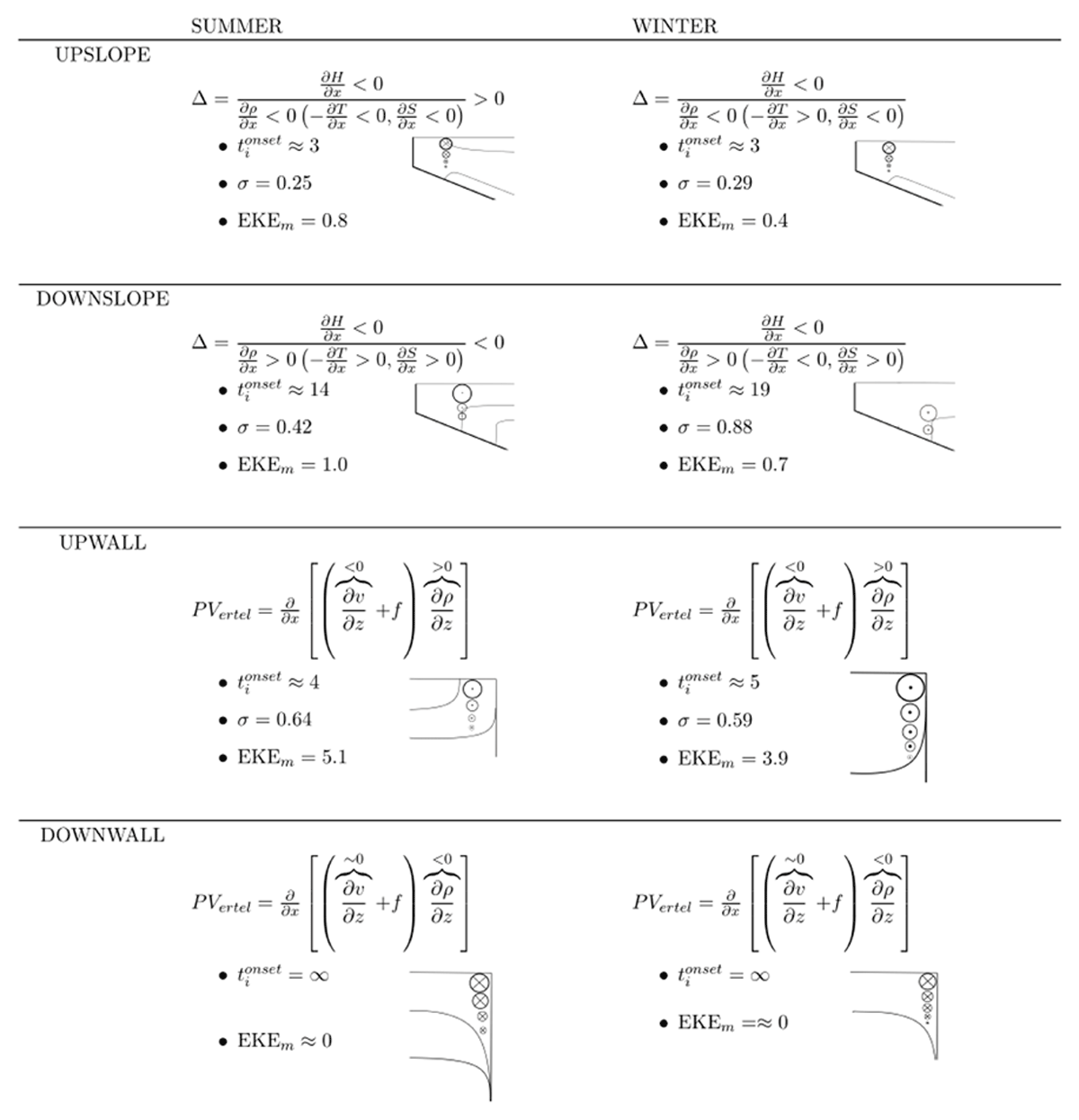
Figure 4
A schematic summary of the instability diagnostics for the different model configurations. EKE is given in 10–6 m2 s–2. Growth rate in day–1. See text for details.
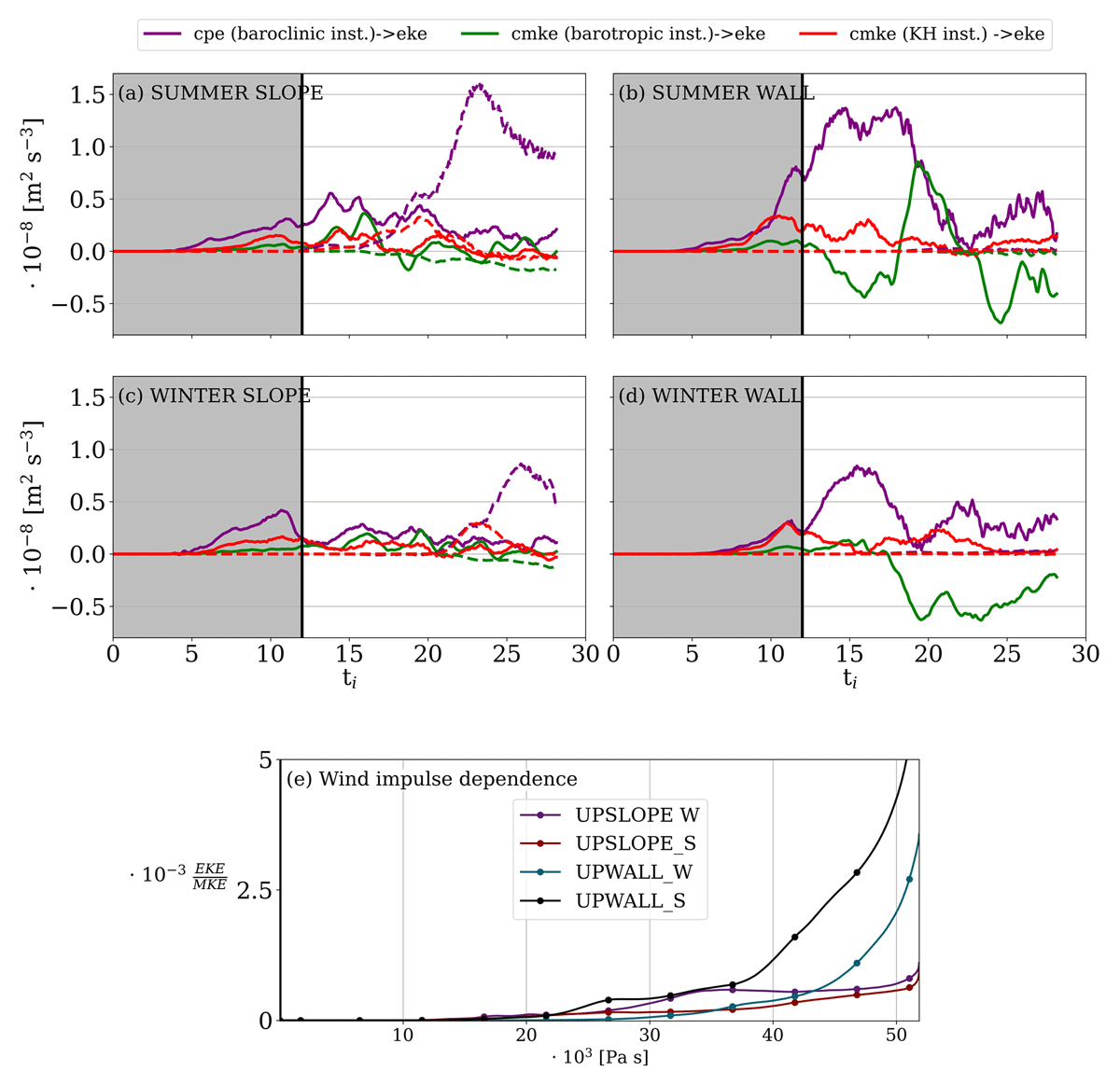
Figure 5
Energy conversion rates. Purple: CPE (PE to EKE, baroclinic instability), green: horizontal shear to EKE (barotropic instability), red: vertical shear to EKE (KH instability). (a and b): Summer SLOPE and summer WALL; (c and d): winter SLOPE and winter WALL. Solid and dashed lines show upwelling and downwelling, respectively. Shaded grey area marks the active phase. (e) Ratio of EKE to MKE (lower panel, c–d) on the wind impulse during the active phase. Dots mark inertial periods.
The conversion of PE to EKE (cpe), associated with the baroclinic instability, dominates the energetics for UP-, and DOWNSLOPE as well as UPWALL, while DOWNWALL does not exhibit instability. The onset of instability is approximately the same for UPSLOPE summer and winter (, corresponding to a wind impulse of ~12000 Pa s, see Figure 5e) the onset is approximately at the same time for UPWALL summer () and for UPWALL winter the onset is postponed to , corresponding to a wind impulse of ~22 500 Pa s. In all upwelling simulations the onset occurs already during the active phase.
The onset for DOWNSLOPE occurs later during the passive phase ( in summer, in winter) because of the weaker stratification and wind shear during the active phase. The longer onset makes DOWNSLOPE instability less likely to occur in the WGB than UPSLOPE as the northeasterly winds are less frequent (~10% time) than southwesterly winds (~30% time) while the winds tend to change direction often on short time scales (Figure 1c–d). The onset of instability for upwelling is directly related to the wind impulse during the active phase: the flow gets unstable for Pa s for all flow regimes for the given geometry and stratification (Figure 5e).
The onset of baroclinic instability is associated with the off-shore migration of the coastal jets for all unstable regimes (UPSLOPE, UPWALL and DOWNSLOPE; Figure 3, middle panels) and development of frontal recirculations. The contribution of the baroclinic component to the total flow at the later time during the active phase is shown in Figure 6.
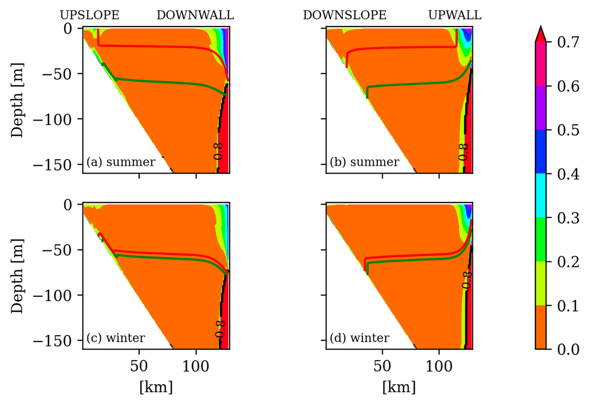
Figure 6
The ratio of the baroclinic component vbc (total subtracted the depth-average) to the total alongshore velocity v at ti = 8 for summer UPSLOPE-DOWNWALL and DOWNSLOPE-UPWALL (a–b) and winter UPSLOPE-DOWNWALL and DOWNSLOPE-UPWALL (c–d).
Clearly, while the circulation on the slope is more barotropic (see also Section 3.1), the circulation at the wall is more baroclinic. The baroclinic flows on both sides are coupled to both, thermocline and halocline, in summer (in winter both interfaces nearly coincide). Thus, the presence of the displacement of the summer surface thermocline intensifies the instability (by increasing the ), but it is not necessary for the development of instabilities due to the halocline. The maximum of EKE decreases by almost a factor of 5 from WALL to SLOPE and by a factor 2 from summer to winter because of the weaker winter stratification and thermal wind (not shown).
The baroclinic instability on the slope is further assessed using the ratio of the bottom slope to the isopycnal slope () as in the Eady problem with a sloping bottom (Isachsen, 2011; Stipa, 2004; Zhurbas et al., 2006). For the flow is unstable with a fastest growing mode of (1.61 for the Eady model). For no unstable solutions can be found, for (opposing isopycnal and bottom slopes) the flow is unstable and the growth rate decreases with , while there is a strong stabilization of long waves and the short-wave cut-off moves to even shorter waves (see Stipa (2004), their fig. 2 and Isachsen (2011), their fig. 1]. In our simulations, . For UPSLOPE, , so and the flow can be stable or unstable depending primarily on the strength of the upwelling (wind forcing) and stratification; since in summer and in winter, implying that upwelling on the slope is more prone to instability in summer than in winter for a given wind magnitude due to the outcropping summer thermocline and the unstable wavelength compares to Rbc, and the estimated growth rates are about 4 day (Figures 4, 5). For DOWNSLOPE, so and the system is always unstable, but because of the seasonality in temperature stratification, , the growth rate (onset) of instability is larger (faster) for the summer, consistently with our simulations (Figures 4, 5), and the short waves are more unstable.
We zoom into the flow under baroclinic instability on the slope in summer in Figure 7 (UPSLOPE) and Figure 8 (DOWNSLOPE) showing the cross-shore density gradients (thermal wind, panels a) and the Ertel PV field (Equation 20, panel b) a couple of inertial periods after the onset of instability.
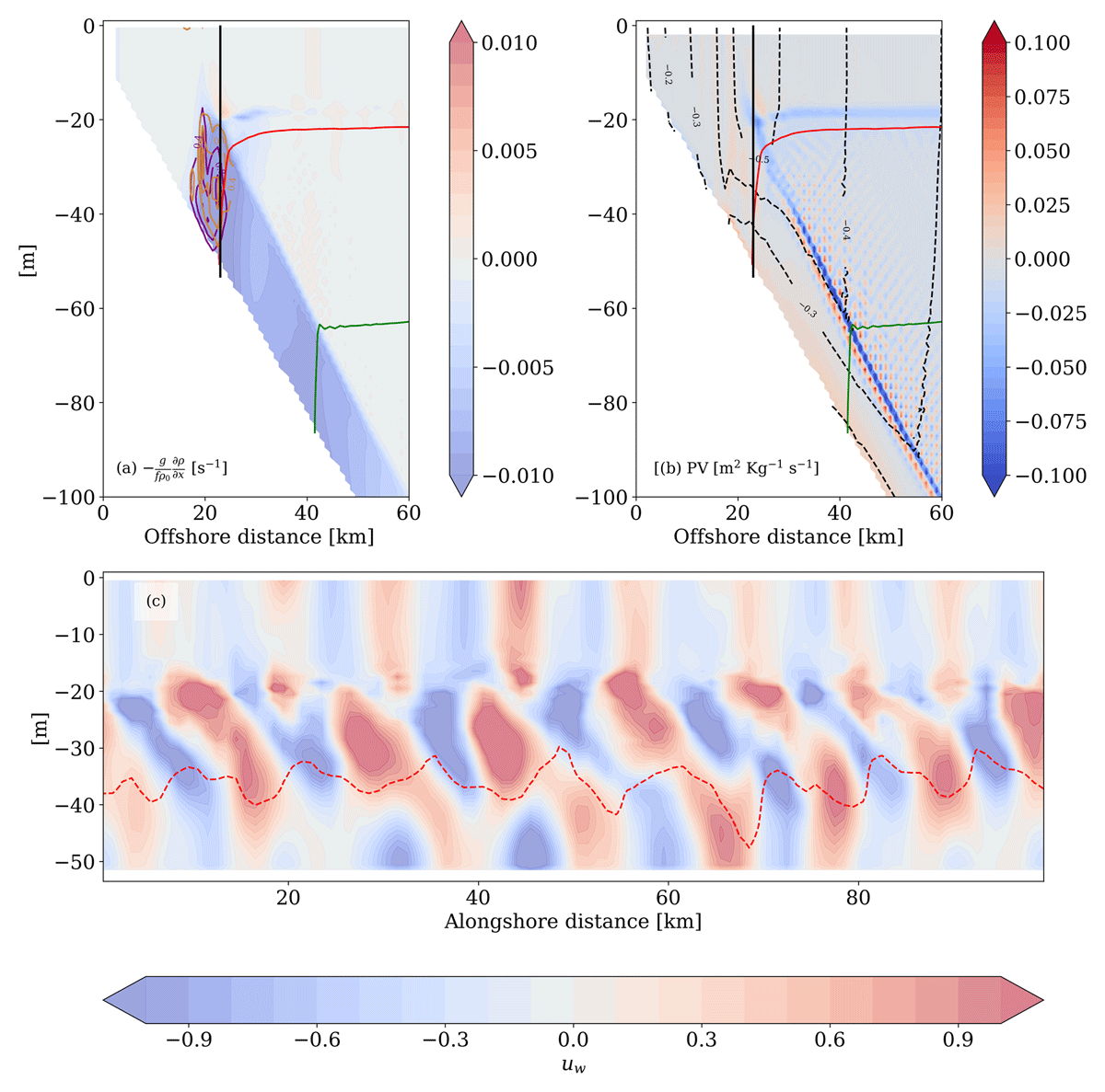
Figure 7
Instability diagnostics after the onset of instability (ti = 6) for UPSLOPE, summer. (a): Thermal wind overlapped with contours of cpe (purple lines) and cmke (green lines). Contour lines show the interval (0.4, 1.6) · 10–8, with every interval given by 0.4 · 10–8. Thermocline and halocline are given by the dashed red and green lines, respectively. The vertical solid black line marks the frontal jet location alongshore section in (c) is taken. (b) PV field contours of alongshore velocity (coastal jet; black lines). (c) Alongshore section of normalized cross-shore velocity uw at the frontal jet location (black solid line in (a)).
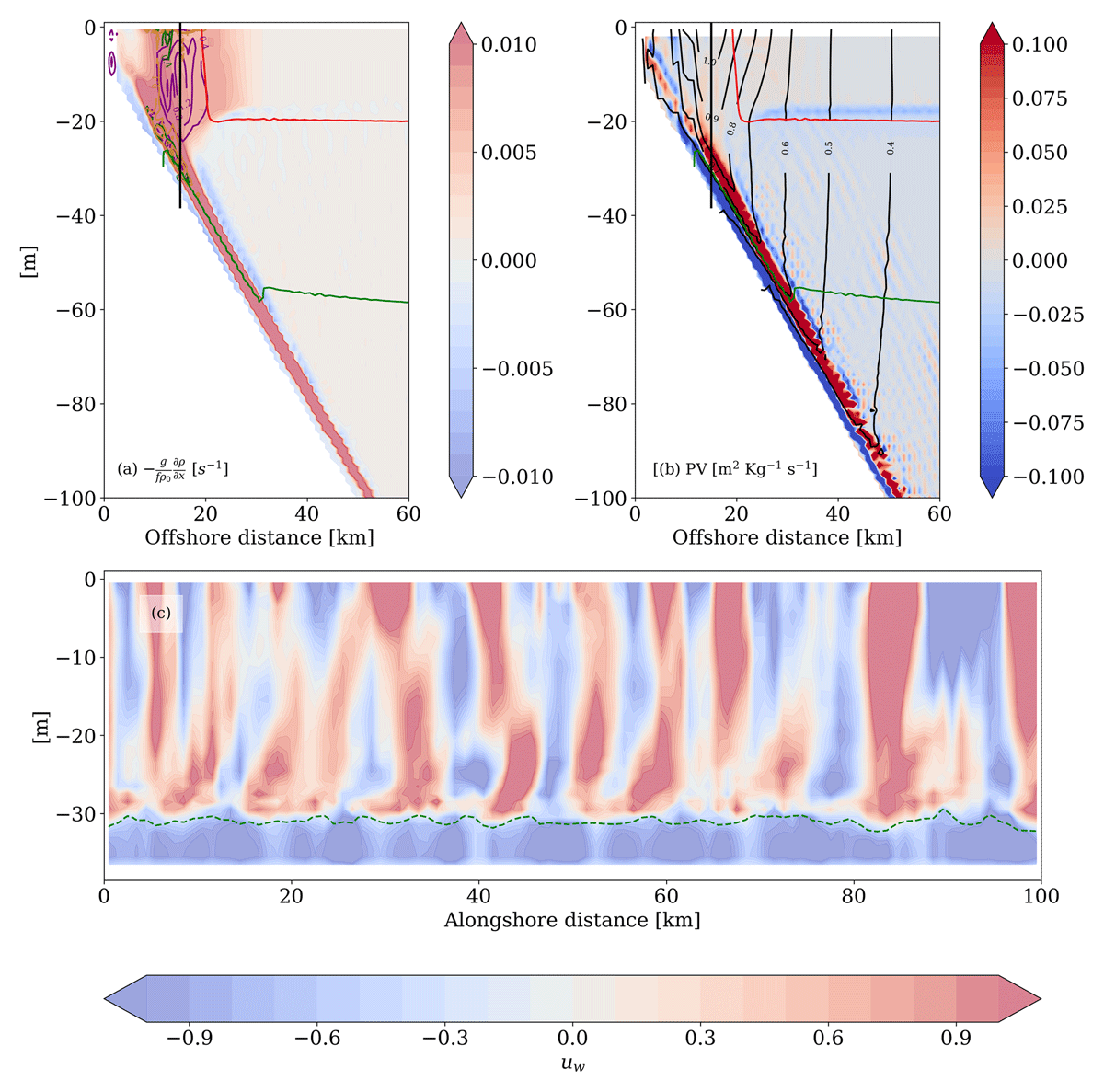
Figure 8
Same as Figure 7 but for DOWNSLOPE, summer, ti = 18.
The horizontal density gradient (thermal wind) is negative (positive) for UPSLOPE vs. DOWNSLOPE and since the Ekman circulation is reversed, the PV changes sign (a necessary condition for the baroclinic instability) from positive to negative within a broader region along the slope bounded by the jet (front) maximum and the halocline (a region of baroclinic flow, see Figure 6). The maximum cpe is localized at the jet location due to the strong thermal wind there (sufficient condition) in both cases, however, while for the UPSLOPE this maximum is above the boundary layer, while for DOWNSLOPE it is within. In the result, the instabilities marked by the cross-shore velocity changes (panels c) develop above the bottom boundary layer for UPSLOPE already during the active phase, while the bottom boundary layer upwelling flow continuously refurnishes the cross-shore gradient and the thermal wind; this boundary flow diminishes in the passive phase making the instability waves extend to the bottom (not shown). For DOWNSLOPE the instability develops during the passive phase when three-layer structure associated with a detachment of the jet spans the bottom boundary layer. This is consistent with Stipa (2004) who found that in case of (DOWNSLOPE) the long waves are confined to the lower boundary. For increasing wavenumbers (shorter waves), the upper boundary comes into play, triggering interaction between the perturbations on both boundaries and their growth in time, because the shear maintains their phase difference while the mutually induced velocity field tends to diminish it. If bottom Ekman pumping is applied in this case, the short-wave bottom-trapped Eady solution is barotropised and becomes strongly decaying by increased Ekman pumping, explaining why the onset of instability for DOWNSLOPE in our simulations is postponed to the passive phase. The DOWNSLOPE pattern is similar in winter albeit with weaker thermal wind and PV gradients since the winter thermocline (colder water at the surface) weakens the salinity stratification and is also located close to the halocline, resulting in a deeper mixed layer (not shown).
For the wall side, the baroclinic instability is referenced directly to the PV gradient (Vallis, 2019). The vertical component of relative vorticity in Ertel PV (Equation 20) dominates and thus the cross-shore gradient yields . Since is not changing sign close to the wall during the period when the instabilities’ set on (Figure 3, first row), the necessary condition for the instability can only be satisfied for UPWALL if and when changes sign when the jet detaches from the wall (Figure 3, third row). The signs are reversed in DOWNWALL, but the same argument holds; DOWNWALL does not exhibit detachment (Figure 3, third row) which implies that it is always stable, consistently with energy diagnostics (Figure 5e–h). See Figure 4 for the summary.
3.4 Coastal eddy field
Baroclinic instability results in meandering of the coastal jet and formation of an eddy field. Because instabilities associated with the relaxation of the downwelling front occur without any signature on the surface density, following Durski and Allen (2005) we choose to use the depth-averaged cross-shore velocity (transport per unit length in along-shore direction) (Figure 9a–f). In a uniform alongshore channel, the depth-averaged cross-shore velocity does not depend on time, any deviation in time would mark the presence of instabilities (see sum of equations 25 and 28). Note that the cross-shore velocity shows a vertical structure (Figures 7–8) due to growing perturbations (Stipa, 2004) as well as detachment of coastal jets in the relaxation phase (Figure 3). This vertical structure is averaged out in Figure 9a–f, which are used here to quantify the integrated cross-shore transport due to turbulent features generated by the instability.
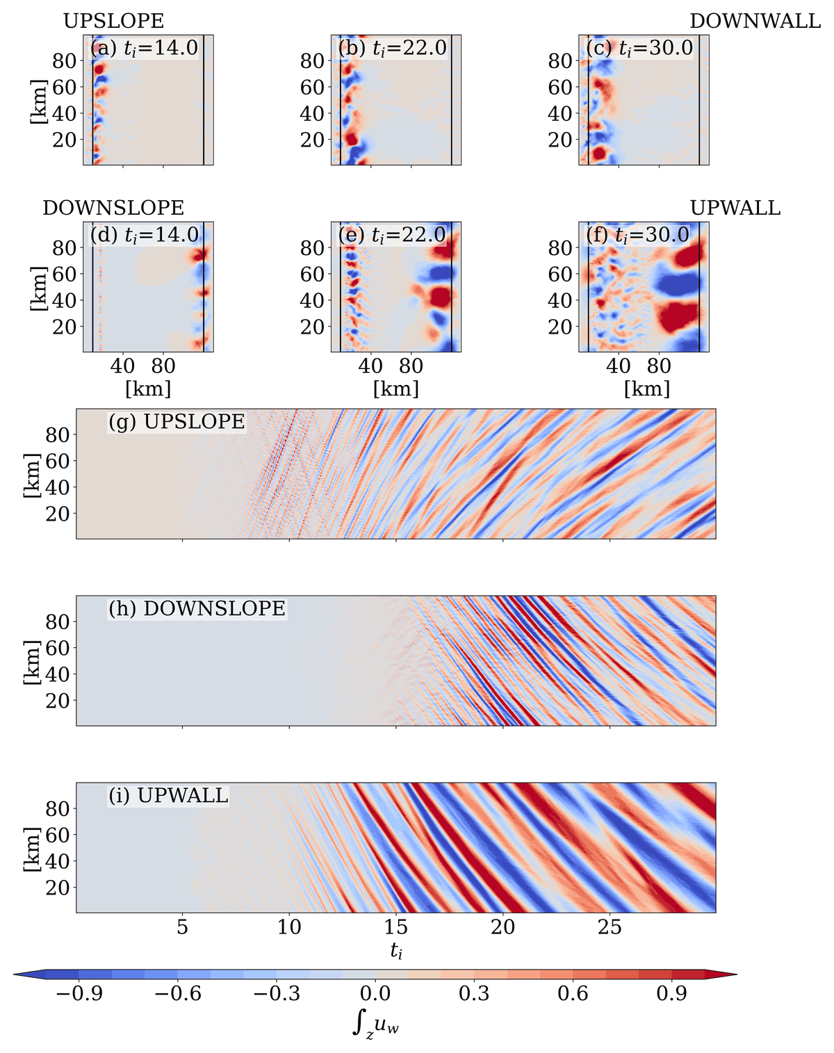
Figure 9
A top view of the depth-averaged cross-shore velocity field for positive wind stress (first row, a–c) and negative wind stress (second row, d–f) at ti = 14, 22, 30 in summer. Hovmöller diagrams for the depth averaged cross-shore velocity field at the location marked by the solid black line in panels above marking the location of the upwelling and downwelling front at the onset of instabilities: (g) DOWNSLOPE, (h) UPWALL, and (i) UPSLOPE.
The dominant wavelength is estimated from the first zero crossing of the autocorrelation function of Uw with distance off-shore. For the UPWALL, the unstable wavelength growths from about Rbc to 50 km. The presence of the slope reduces the unstable wavelength ().
Those differences are qualitatively consistent with the results from the two-layer model of baroclinic instability. The absence of the sloping bottom maps onto zero topographic , implying that there is only a high wavenumber cutoff [(Philips model, (Vallis, 2019))] and the size of unstable waves is restricted solely by the geometry of the channel (about 50 km in our simulations). On the sloping bottom, the most unstable wavelength for UPSLOPE and for the DOWNSLOPE the most unstable wavelength is in the short wave range and depends on exact value of (Isachsen, 2011; Stipa, 2004).
Hovmöller diagrams (Figure 9g–i) show propagation of disturbances alongshore in time while they grow in size. In the absence of the mean flow, unstable waves on the slope would propagate with the shallow side to the right (negative velocity alongshore) due to the topographic beta effect which superimposes on the advection by coastal jets, which (vertically averaged) velocity drops by about half over the passive phase. For UPSLOPE (Figure 9g), the propagation is initially dominated by the advection by the positive coastal jet resulting in a positive alongshore propagation speed 100 km/3Ti ≈ 0.6 m/s, which implies a fast transport due to upwelling jet out of the WGB. During the passive phase the jet fades away and the slope effect yields a slow net positive propagation (50 km/5Ti ≈ 0.2 m/s). For the DOWNSLOPE, the propagation on the slope has same direction as the coastal jet (negative) but the instability sets in well into the passive phase when the jet is already weakened resulting in net negative propagation of about –0.4 m/s at ti = 15 and dropping to –0.3 m/s at the end of the simulation, i.e., continued significant transport southward of the domain long after the wind has ceased. Note also that there is a signature of small scale, weaker instabilities on the inner shelf for both DOWNSLOPE and UPSLOPE. For UPWALL, there is no topographic beta effect and the instabilities are advected by the negative jet alongshore with a of 0.8 m/s at the beginning of the passive phase and then slow down toward the end of the passive phase to 0.3 m/s as they also interact with disturbances from the slope side propagating offshore.
3.5 Implications for mixing
The role of coastal upwelling for mixing in the Baltic Sea have been studied previously in an idealized configuration (Zhurbas et al., 2006) and its sub-basins [e.g., Gulf of Finland, (U. Lips et al., 2017; Väli et al., 2017; Zhurbas et al., 2008), but no studies have considered WGB so far. We quantify the implications for momentum and tracer mixing using the vertical eddy mixing coefficient KV (state-dependent output from the model KPP parameterization scheme) and the surface cross-shore eddy salinity flux , where indicates the cross-shore mean (Figure 10). Large values of KV () prevail in the surface and bottom Ekman boundary layers during the active phase, with a thicker bottom layer and higher values for the DOWNSLOPE (due to a lower stratification there) compared to UPSLOPE (Figure 10a and d). While for the UPSLOPE the high vertical mixing layers first thicken at the unstable frontal jet and then successively fade away during the passive phase (Figure 10b–c), they persist for DOWNSLOPE throughout the simulation time (Figure 10e–f). A striking result is that for DOWNSLOPE, the high KV values are found on the inner shelf, suggesting that the downwelling jet on the sloping bottom may play a prominent role in determining the vertical mixing of the broad inner shelf parts of the WGB. The DOWNWALL has no clear signal in KV (Figure 10a–c) while baroclinically unstable jet and eddies for the UPWALL come across as centres of elevated vertical mixing KV () consistent with the ‘chimney effect’ of baroclinic eddies for vertical mixing found in earlier studies (Koszalka et al., 2010).
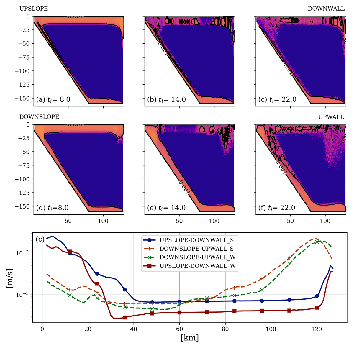
Figure 10
Alongshore averaged vertical viscosity coefficient from KPP scheme for UPSLOPE-DOWNWALL (upper panel, a–c) and for DOWNSLOPE-UPWALL (lower panel, d–f) at selected times ti = 8, 14, 22. Solid black line marks the contour of 10–3 m2 s–1. (g): Surface cross-shore eddy salinity fluxes averaged in the alongshore direction and between t = 10 t2 and 20 t2.
On the contrary, the surface horizontal mixing is generally low during the active phase (not shown) and gets successively elevated due to instabilities and baroclinic eddies (Figure 10g). This is consistent with observations and modeling results about the important role of unstable jets and baroclinic eddies for cross-shore transport in other regions (Isachsen et al., 2012). The cross-shore eddy fluxes are one order of magnitude larger for UPSLOPE and UPWALL (due to baroclinic instability with larger unstable wavelengths) compared to DOWNSLOPE (baroclinic instability with smaller wavelengths, Figure 9) and DOWNWALL (no instability) and concentrated within the first 20 km from the coast, i.e., marked by the location of the coastal jet (Section 3.2). Thus, while the northeasterly wind regime with downwelling on the Swedish coast and upwelling on Gotland side is a much more rare event in the WGB (10% time compared to about 30% for upwelling; Figure 1c), it is a more effective ‘bottom vertical mixer’ (with implications for the bottom boundary layer biogeochemistry and coastal hypoxia (Fredriksson et al., 2024))]. On the other hand, the southwesterly wind regime (upwelling on the Swedish coast and downwelling on the Gotland side) are more effective ‘surface horizontal mixers’ [with implications for, e.g., algae blooms and air-sea exchange; (I. Lips and Lips, 2008); (Dabuleviciene et al., 2020); (Norman et al., 2013)).
3.6 Topographic effects and relevance of idealized simulations
So far we focused on simulations with a constant slope on the Swedish coast. In reality, the slope is not uniform but steepening from south towards the Landsort Deep. However, for the range of observed slopes Bu is always small (between 0.2 and 0.4), barely modulating the contribution of the boundary layer to the offshore transport, so our results about the main features of the coastal circulation hold over.
The bathymetry of the WGB is complex, resembling a sinusoidal shape but with a deep depression of the Landsort Deep in the northern part of the domain and a few larger bays and gulfs (Figure 1c). As a next step in refining the representation, we considered a sinusoidally varying slope topography (Section 2.3). It resulted in a meandering of the coastal jets due to squeezing and stretching of the water column, but the qualitative picture of baroclinic instability did not change (Figure A2). Several other studies addressed the interaction of locally varying bathymetry with upwelling in similar idealized configurations. For example, Saldías and Allen (2020) studied the upwelling on the shelf with a deep canyon and open sea boundary. The presence of a submarine canyon imprinted on the circulation and coastal upwelling structure close to the canyon; part of which can be associated with squeezing and stretching resulting in jet meandering. The baroclinic instability was still the main instability mechanism while the presence of the canyon increased the wavelengths downstream. They attributed part of the observed variability to the presence of coastal trapped waves (CTWs) (i.e., Kelvin-like waves propagating along a sloping coast) (Walin, 1972a, b). Also Fennel and Seifert (1995) addressed the interaction of such waves with upwelling in the southern Baltic Sea with idealized model configuration but did not quantify them in detail. The variability in hydrographic observations on western Gotland’s coast have been traced back to propagation of CTWs excited at the southern tip of Gotland (Pizarro and Shaffer, 1998). Fennel et al. (2010) studied the interaction of Kelvin waves generated at the northern and southern tip with upwelling around Gotland. The upwelling signal is amplified or reduced by Kelvin waves at different locations around the island, depending on local stratification and water depth which determines the wave dispersion and damping. The (frequent) downwelling signal from the western part of the island is propagated by the waves to and along the eastern side reducing the upwelling signal there, but the opposite is not occurring on the western side due to stratification-depth conditions there. Our idealized simulations are not designed to study the dynamics of CTWs in the WGB. A follow-up study should address the impact of locally complex bathymetry and the presence of Landsort Deep in the WGB, including the interaction with CTWs to identify locations of persistent and wave-modified upwelling/downwelling patterns and their impacts on biogeochemistry in the WGB. Our idealized configuration does not fully represent the role of inertial and inertial-internal waves in the dynamics because of the lack of continuous variations in wind forcing. These waves are transient phenomena in our simulations and the inertial frequency band (corresponding to periods of 12–16 hours) makes up to 13% of the total variance for the cross-shore velocity component at the depth of the summer thermocline, and below 5% for other components). Inertial and internal waves were however found significant in the observations of upwelling (Walter et al., 2016), idealized upwelling simulations with forcing oscillating in time (Brink and Lentz, 2010) and idealized simulations of ocean eddy field forced with spatially-varying winds (Koszalka et al., 2010). Recent observational and modelling studies suggest that horizontal transport due to the wind waves is important in coastal seas (Stanev et al., 2019; Staneva et al., 2021). Future more realistic and focused numerical studies are needed to assess the wave dynamics and wave-induced transport in the WGB.
Another important aspect not considered here is the modulation of Ekman dynamics by surface buoyancy fluxes on daily to sub-seasonal time scales. A modeling study addressing this issue was done by Nerheim and Stigebrandt (2006) to explain variability in observed buoy data. Including buoyancy flux would be a necessary step towards more realistic studies of the dynamics in the WGB.
The idealized simulations can help to isolate the underlying instability dynamics and associated time and space scales. It is not easy to isolate the upwelling and downwelling in observations because of the transient nature of the wind events and interaction with complex topography, coastally trapped waves, river run-off and air-sea interactions. We downloaded and inspected GHRSST (https://www.ghrsst.org/), and MODIS data (https://oceandata.sci.gsfc.nasa.gov), but the upwelling and downwelling development on two sides of the WGB is hard to study systematically using satellite products because of the frequent cloud coverage and few available swaths over the area. Moreover, downwelling is not easily detectable in SST images, and upwelling is hard to detect during winter. Even during the summer, the detectability of the upwelling may be limited, depending on the intensity and duration of the wind event that determines the outcrop of the summer thermocline (Section 3a–b). Using reanalysis products circumvents the issue with the cloud cover and provides velocity fields, but is instead prone to errors due to limited model resolution (nominal resolution of 1 nm = 1,852 km) and data assimilation.
Nevertheless, in lieu of satellite data of sufficient coverage and resolution, the reanalysis products can help to analyze velocity- and derived quantities and regionalize our idealized results as well as to discuss their limitations in representing the more realistic representation offered by the reanalysis. To exemplify the representativeness of our idealized simulations, we choose a north-easterly wind event in August 2021 evidenced in wind observations (Figure 11a) and show results from reanalysis at about ti = 16 duration of the wind event (SST and surface relative vorticity; Figure 11b and e). This meteorological situation is less frequent in WGB (north-easterly winds occur with about 10% frequency, Figure 1c) and corresponds to our idealized DOWNSLOPE-UPWALL configuration where the jets on both basin sides are unstable (with instability onset times of about 14 and 4 inertial periods for DOWNSLOPE and UPWALL, respectively, Figure 4) and an eddy field spanning the whole basin develops from the unstable UPWALL coastal jet (Figure 9).
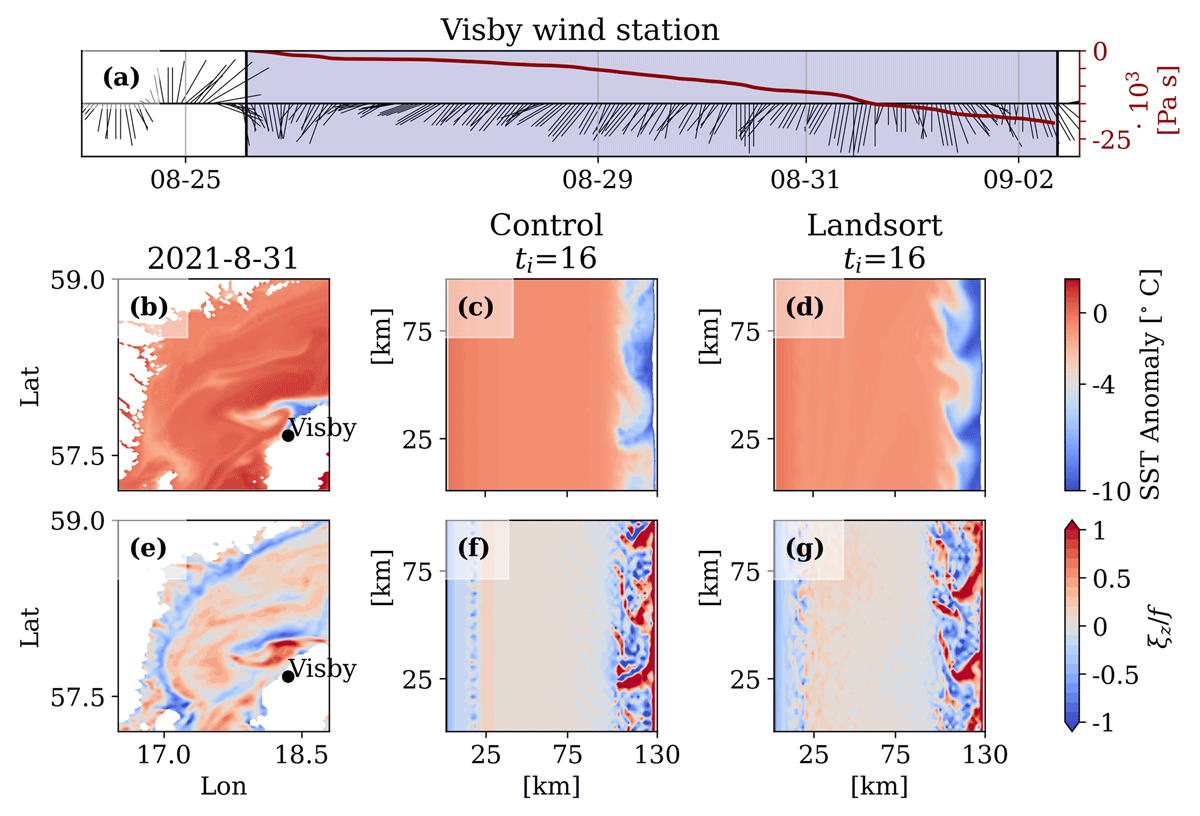
Figure 11
(a) Stickplot for wind speed and direction measured at the SMHI meteorological station in Visby during a northeasterly wind event in August 2021 (downloaded from http://opendata.smhi.se/apidocs/metobs/index.html, assessed on 29th April 2024, 14:58:24). On the right-axis, the alongshore wind impulse has been plotted (computed using equation 2 and by rotating the wind vector of 45° which is an approximate the coast direction and the N-S). Panels (b) and (e) show, respectively, the SST anomaly ([°C]) from the domain average on the 26th of August 2021 (prior to the upwelling event) and the vertical component of the relative vorticity at the surface ( derived from sea state forecast for the 2021-08-31 (https://marine.copernicus.eu/, DOI: https://doi.org/10.48670/moi-00010, accessed 2023-07-18 14:38 UTC). Panels (c) and (f) show the model anomaly surface potential temperature from the domain average at and the relative vorticity from the channel with uniform bathymetry (DOWNSLOPE-UPWALL summer), and the same field are plotted in (d) and (g) for simusoidally varying bathymetry (LANDSORT DOWNSLOPE-UPWALL summer) for .
Figure 11c and f show, respectively, the SST anomaly and the relative vorticity from our idealized simulations with summer stratification for uniform bathymetry, and panels d and g show the same for the sinusoidally varying bathymetry (LANDSORT). The SST anomaly is computed from the mean in the domain before the onset of upwelling (26th August 2021). Consistent features between the reanalysis and idealized simulations are: 1) a downwelling jet on the eastern (DOWNSLOPE) side indiscernible in SST field but marked by negative values in the relative vorticity because of squeezing over the sloping bottom [e.g., (Zhurbas et al., 2006) and showing signs for onset of instability after about two weeks with a few kilometer-scale meanders, 2) unstable eddy visible in SST and relative vorticity field with about 25 km length scale formed due to instability of upwelling jet on the western (UPWALL) side (for a wind impulse of about 11,000 Pa s; in accordance to our results in Figure 5e).
Note that the observed wind is varying during the event duration so the observed wind impulse is lower than in our idealized simulations (Figure 1d), but it is sufficiently large to generate instabilities in accordance to our simulations (EKE/MKE >0, see Figure 5e) while they are, as expected, less intense (EKE is smaller in reanalysis as only one eddy feature is observed). There are also differences, however. In the reanalysis, the downwelling jet seems to be advecting a cold water anomaly into WGB from the northern direction disrupting the downwelling signal inside the basin, there is signature of runoff and small scale flow features at the eastern coast, and the coastal jets on both sides of WGB interact with the flow associated to the Oland Island located in the south. These interactions cannot be captured in our idealized simulations with periodic north-south boundaries and idealized coasts; however, this comparison shows that the salient dynamics of coastal jets and related instabilities is well represented in idealized simulations on length scales comparable to, and larger than, the baroclinic Rossby radius and time scales longer than inertial.
To address the relevance of an idealized simulations of the WGB channel of a finite width, we investigate the time evolution (Hovmöller diagrams) of the velocity components (Appendix Figure A3, top three rows). These show evidence for interaction of the coastal flows across the domain after the onset of instabilities, involving both the subinertial dynamics and inertial waves (evident mostly in the cross-shore velocity component). We quantify further the interaction of coastal jets due to nonlinear dynamics by alongshore- and vertically averaged alongshore velocity tendency due to cross-shore advection during one inertial period (, , bottom row in Figure A3). This interaction leads to a change in alongshore velocity of the order of a few cm/s during one inertial period and for DOWNSLOPE-UPWALL, it extends across the domain after the instabilities develop. Note that the interaction between the flows on two sides of the domain implies that it is not straightforward to replace our channel configuration by separate model configurations of coastal jets on the two sides of the channel as in e.g., Brink (2016). Appropriate open boundary conditions would be needed not only to cope with the artificial reflection of outgoing waves offshore but also tackle the non-zero geostrophic flow in the middle of the domain (see also numerical experiments and discussion in Nycander and Doos (2003)). The MITgcm has a choice for prescribing the flow at the open boundary following Stevens (1990) that could possibly be adopted to this case in a future work.
3.7 Sensitivity studies
We ran a simulation with a higher horizontal resolution (500 m), however, this showed no notable changes in the coastal jet and instability dynamics, implying that the nominal 1 km resolution was sufficient to represent the baroclinic flows given the regionally typical winds and stratification (). We ran simulations with the quadratic bottom drag coefficient () to assess the sensitivity to the drag parameterization. The formation of the boundary layer and pycnic displacements showed no significant change, nor did the instability dynamics. The bottom velocity however, became stronger at the end of the active phase and the decay of the mean flow was slower in the passive phase for the quadratic drag case compared to the linear one. The estimated buoyancy arrest time scales (Equations 31–32) are even longer ( for UPSLOPE, for DOWNSLOPE) for the quadratic bottom drag. It is to be noted that the buoyancy arrest time scales depend on the product of the drag coefficient and stratification (in a square-root manner for upwelling, and linearly for downwelling; Equations 31–32), which implies a sensitivity to the value of Cd, although one can expect that the Cd and N are not independent (stronger friction would lead to a weaker bottom flow and more quiescent conditions and thus stronger stratification). To test this, we also run a simulation with much higher , and we did not observe a substantial change in the dynamics, consistently with Brink (2016).
A sensitivity study to the vertical mixing scheme for coastal upwelling has been done by Durski and Allen (2005) who did not observe remarkable differences between simulations run with the Mellor–Yamada and the KPP schemes. We expect that their result would carry to our configuration where most of the cross-shelf transport occurs in the bottom boundary layer (), with only a minor contribution from the interior and surface mixed layer (where one would expect largest differences due to vertical mixing schemes).
4 Conclusions
In this study, we considered transient upwelling and downwelling dynamics in a channel-like domain in the Baltic Sea (Western Gotland Basin, WGB) featuring a sloping bottom on the west (Swedish mainland) side and a steep bathymetry on the east (Gotland Island) side. We applied typical regional wind conditions (alongshore gentle breeze of a few days duration, ‘active phase’) followed by an unforced relaxation period (‘passive phase’) and varied between the summer and winter stratification. To our knowledge, this is the first high resolution modelling study of transient upwelling and downwelling in such a configuration. We also derived an analytical solution for coastal jets in a two-layer channel with vertical walls for comparison with model simulations to assess the role of sloping geometry and seasonally varying stratification.
Although our study builds upon previous idealized studies of upwelling and downwelling (e.g. Brink, 2016; Brink and Seo, 2016; Durski and Allen, 2005; Zhurbas et al., 2008), we complement the research with theoretical considerations based on Csanady (1982); Stipa (2004), and perform an extensive study of instability conditions and scales using energetics and PV- and turbulent transport diagnostics. We find that the unique WGB setting features new aspects compared to the previous literature, in particular the asymmetric response on the two sides of the channel in terms of the lifecycles and stability of the coastal jets that depend on the presence of the sloping boundary on one of the channel sides, the wind direction and in the seasonal stratification. In the regional context, this asymmetry in wind-driven flows in the WGB will be further strengthened given that the winds in the region have a preferred direction (south-westerly) and the duration of transient wind events is often shorter than instability growth time scales on either coastal side. We also find evidence for a cross-shore exchange between the flows on the two sides of the channel, which is not straightforward to reproduce with two one-side model simulations with open boundary conditions.
Our model simulations exhibit coastal trapped upwelling and downwelling jets on both sides of the domain coupled by the interior flow with hyperbolic-shaped interfaces at the coasts, modified by the presence of the bottom boundary on the slope side. The growth of sea surface amplitude is linear in time during the active phase, which is consistent with the theory. The differences between the simulated and analytical solutions are related to the presence of the slope and friction and are small as long as the pycnical displacements are small. The simulated depth of the Ekman layers follows theoretical scaling. Due to the low Burger number (Bu < 0.25), the flow is concentrated in the bottom boundary layer on the slope; this result holds to a range of the slope angles and seasonal stratification in this region and can be used, for example, in models for nutrient fluxes. The buoyancy arrest does not make a remarkable imprint on the dynamics because its characteristic time scales are long (a few days for upwelling, monthly scale for downwelling) compared to the length of a typical transient wind impulse (a few days), and to the onset of instabilities. The timing of the interface outcrop and development of the fronts and their position as well as evolution including the onset of instability are governed by wind forcing and can be predicted from wind impulse. The development of an inner shelf circulation on the onshore side of the slope front, and the shoaling or outcropping warm thermocline during early spring have implications for the oxygen and nutrient fluxes and spring algae blooms.
The barotropic flow is stronger on the slope (Swedish coast) side while the baroclinic energy and thermal wind are stronger on the vertical wall (Gotland) side. The baroclinic instability develops for the upwelling on the slope and wall side and downwelling on the slope side as a result of the offshore displacement of the jet leading to the PV gradient change. For typical transient winds in WGB, up the onset of instability is a few days for upwelling (i.e., already during the active phase when the wind is blowing) and is longer, 2–3 weeks, for downwelling on the slope and occurs in the passive phase when the wind ceases. The onset of instability is related to the wind impulse. The downwelling on the wall (Gotland) side, on the other hand, is always stable. The baroclinic growth rates and wavelengths for our configuration with realistic stratification agree qualitatively with expectations from the theory: they depend on the velocity shear (i.e., the wind stress magnitude and duration which in turn depend on the wind forcing), stratification (with only weak dependence on seasonal variations), and the relative inclination of the bathymetric slope and isopycnals on the slope side (Figure 4).
Given the typical wind conditions (southwesterly winds with 30% frequency, northeasterly winds with 10% frequency) and characteristic transient wind duration of a few days in the WGB, our results imply that a baroclinically unstable upwelling on the slope (Swedish mainland) side (instability onset about 2 days) and a stable downwelling on the wall (Gotland) side invisible from SST imagery (Figure 11a) are favored and can incur up to 30% time. The configuration with downwelling on the slope (Swedish) side (instability onset 2–3 weeks) and upwelling on the wall (Gotland) side (instability onset about 5 days) is less frequent while it can develop an eddy field spanning the whole basin as flows on both sides are unstable and the unstable upwelling on the Gotland side exhibits larger eddy scales. The seasonal differences in stratification have minor effects except for postponing the onset of baroclinic instability for downwelling on the slope (i.e., making it an even rarer event).
The model mixing diagnostics suggest that while downwelling on the slope is a much more rare event in the WGB (northwesterly winds with a 10 % frequency), it is more effective in vertical mixing of the bottom boundary, and might thus trigger strong oxygen and nutrient fluxes on the broad inner shelf along the Swedish coast side of the WGB. Sedimentation in the Baltic Sea is likely to be controlled to a large extent by surface waves, with the exception of locations where other processes may be relevant, (for example, coastal jets) (Jönsson et al., 2005). In particular, for longer and/or stronger wind events, the downwelling over sloping bottom may generate extreme bed shear stresses that can potentially lead to sediment erosion episodes with implications for biogeochemistry of coastal marine ecosystems (Kämpf, 2019).
Future work will address these downwelling impacts on the observed biogeochemical parameter variability and coastal hypoxia in the WGB, in which the physical drivers appear to have a significant role (Fredriksson et al., 2024).
However, more frequent unstable upwelling on slope (southwesterly winds with 30% frequency) and (a rarer) unstable upwelling on the wall side generate strong cross-shore eddy transport in the surface layer, with implications for the spread of algae blooms and air-sea exchanges. Baroclinic eddies emerging due to unstable jets come across as centers of elevated vertical mixing in the surface layer.
Although our study was focused on the WGB the results can be generalized to similar channel basins in the Baltic Sea, for example, the Gulf of Finland or the Gulf of Bothnia, by accounting for local channel geometry, stratification, and prevailing wind conditions. Follow-up studies should consider the interaction of coastally trapped waves and other time-dependent dynamics, with the coastal jets, and the instabilities as well as the impacts on biogeochemistry and primary production in the WGB.
Appendices
Appendix
This illustrative Appendix will show how the flow associated with instabilities evolves for simulation initialized with winter stratification (see Figure A1, Section 2.4) and for alongshore varying bathymetry (see Figure A2, Section 2.3). As discussed in Section 3.6, Figure A3 shows evidence of the interaction of coastal flows across the domain after the onset of instabilities, which involve both the subinertial dynamics and inertial waves, evident mainly in the cross-shore velocity component.
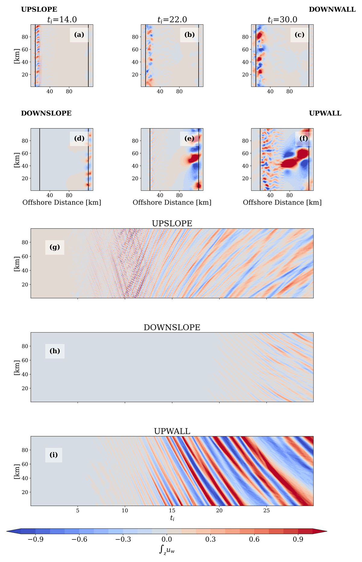
Figure A1
A top view of the depth averaged cross-shore velocity field for positive wind stress (first row, a–c) and negative wind stress (second row, d–f) at ti = 14, 22, 30 in winter. Hovmöller diagrams for the depth averaged cross-shore velocity field at the location marked by the solid black line in panels above marking the location of the upwelling and downwelling front at the onset of instabilities: (g) UPSLOPE, (h) DOWNSLOPE, and (i) UPWALL.
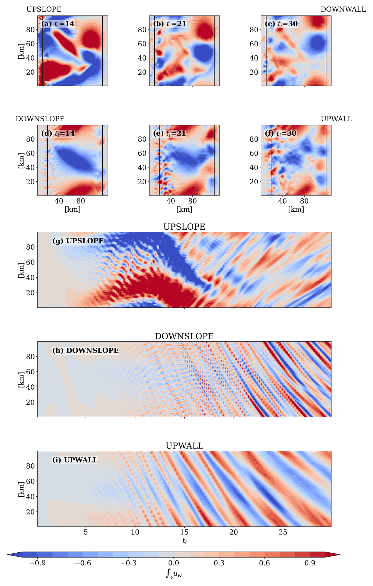
Figure A2
A top view of the depth-averaged cross-shore velocity field for positive wind stress (first row, a–c) and negative wind stress (second row, d–f) at ti = 14, 22, 30 for summer with alongshore varying bathymetry. Hovmöller diagrams for the depth-averaged cross-shore velocity field at the location marked by the solid black line in panels above marking the location of the upwelling and downwelling front at the onset of instabilities: (g) UPSLOPE, (h) DOWNSLOPE, and (i) UPWALL.
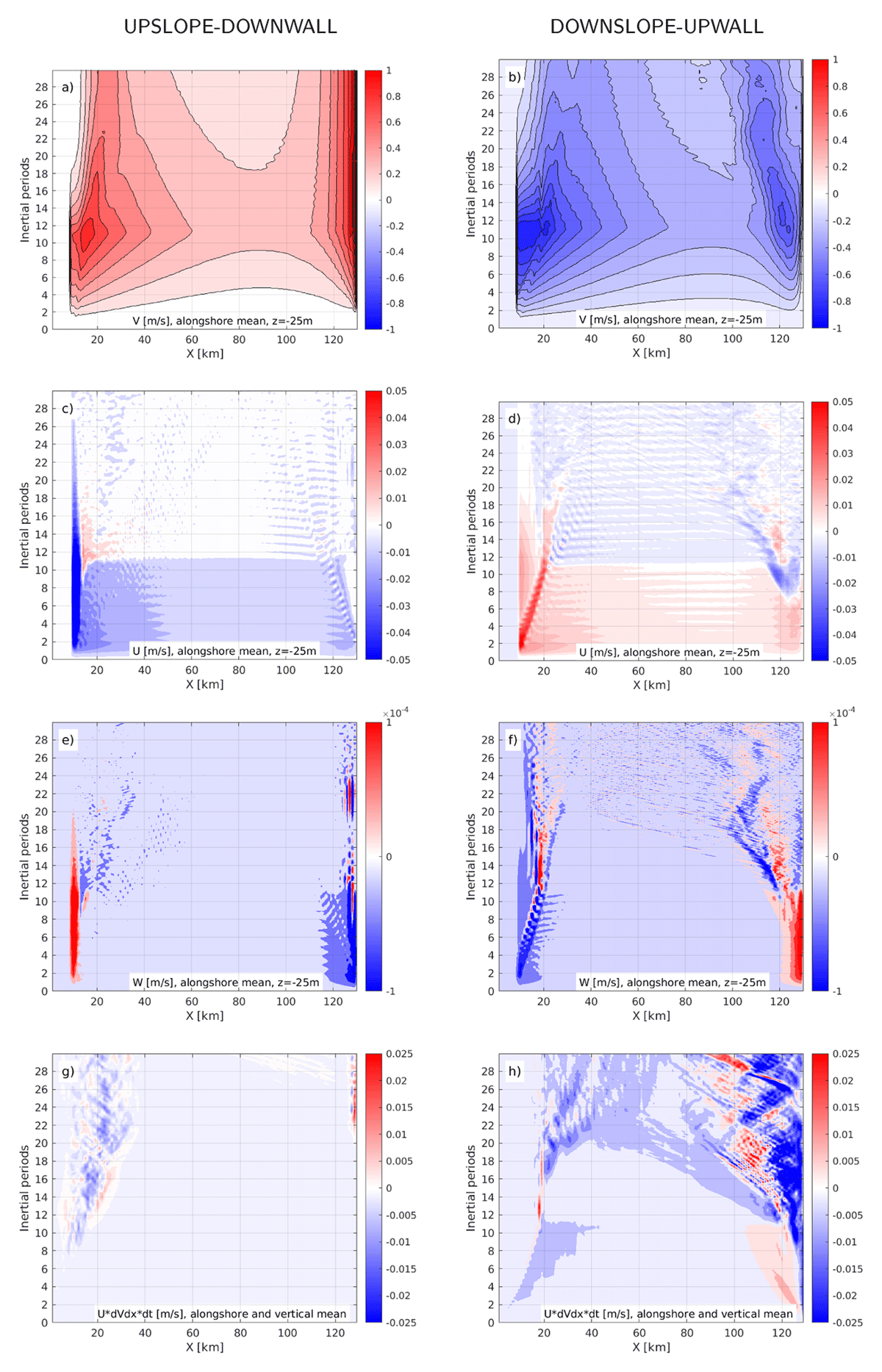
Figure A3
Three upper rows, from top to bottom: Hovmöller diagrams of alongshore averaged: alongshore velocity, cross-shore velocity and vertical velocity, respectively, at the 25 m depth. Bottom row: vertical- and alongshore average of alongshore velocity tendency due to cross-shore advection of alongshore velocity during one inertial period. Left: UPSLOPE-DOWNWALL; Right: DOWNSLOPE-UPWALL. All diagnostics are based on hourly averaged model output from summer simulations.
Acknowledgements
IK would like to acknowledge discussions with Jonas Nycander and Kristofer Döös. We also thank the anonymous reviewers for their insightful and detailed comments.
Competing Interests
The authors have no competing interests to declare.