
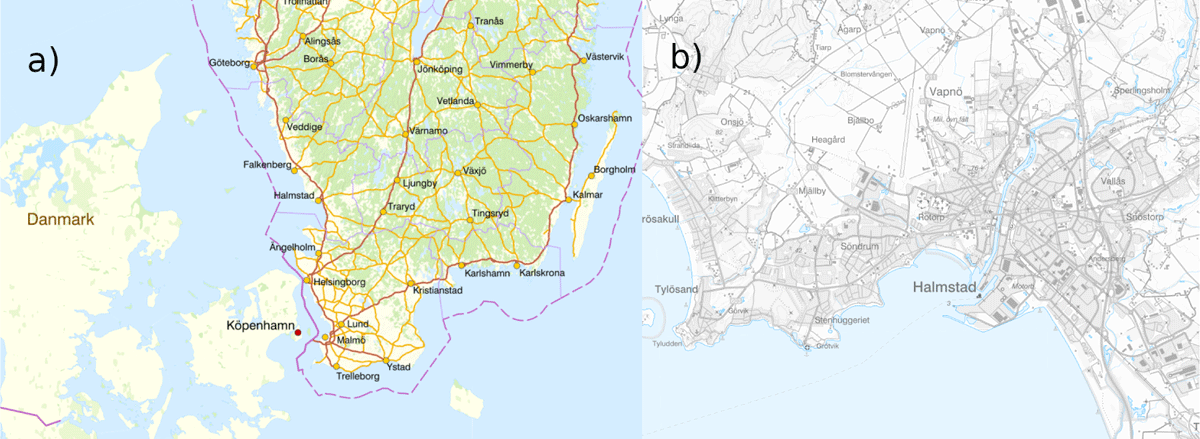
Figure 1
a) cities in southern Sweden and b) city map of Halmstad and the river Nissan that goes through the city centre. a) is taken from the Swedish land survey authority https://minkarta.lantmateriet.se/ and b) from Halmstad municipality https://karta.halmstad.se/.
Table 1
Table of downscaled global coupled models and emission scenarios. The downscaled historical simulations are not the full CMIP5 historical period. Instead they start in the year 1971. All historical simulations, however, end in the year 2005. The RCP scenarios all start in 2006 and end in 2100.
| HISTORICAL | RCP2.6 | RCP4.5 | RCP8.5 | |
|---|---|---|---|---|
| MPI-ESM-LR | X | X | X | X |
| EC-EARTH | X | X | X | X |
| HadGEM2-ES | X | X | X | X |
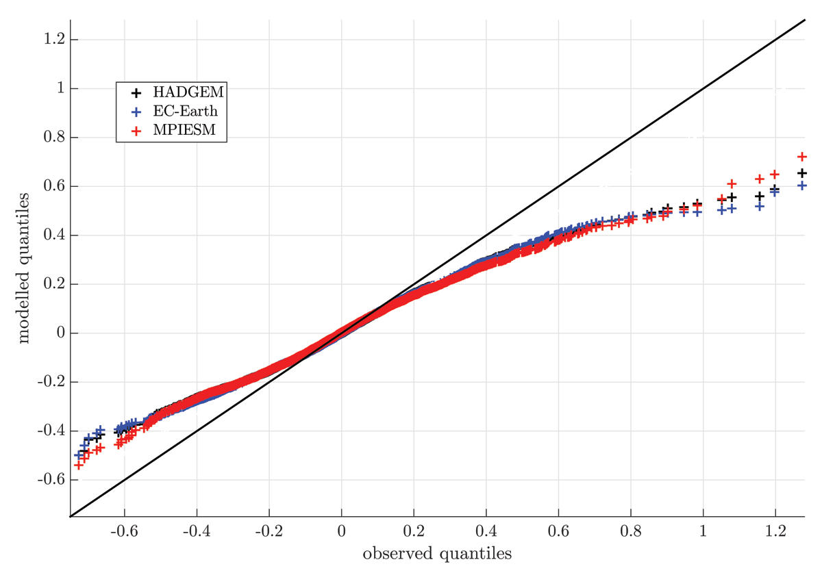
Figure 2
Quantile-quantile plot of sea level observations and modelled sea levels in our three historical simulations, see Tab. 1. All sea levels are daily means. The black line is one to one.
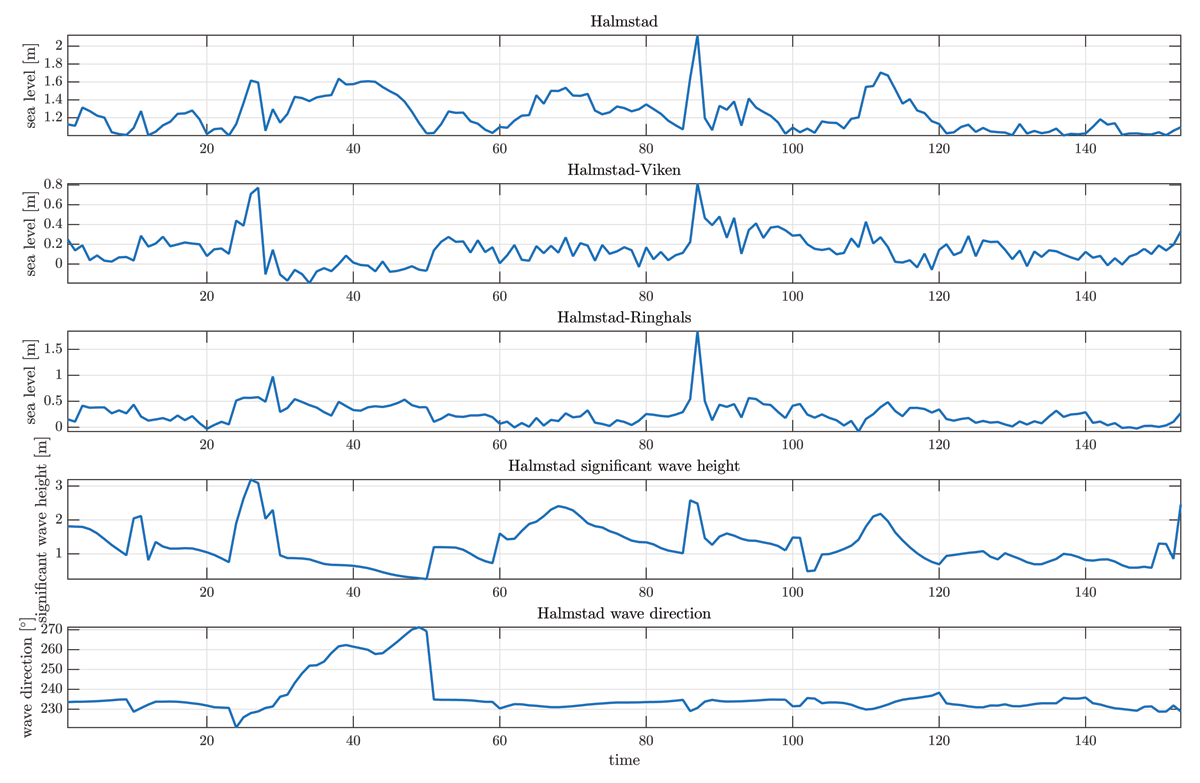
Figure 3
Sea level and wave parameters in Halmstad and at neighbouring stations during the hours in the 2009–2022 period when the sea level in Halmstad exceeded 1 m above the mean. The panels Halmstad-Viken and Halmstad-Ringhals show the sea level in Halmstad minus that in Viken and Ringhals respectively at the times when the sea level in Halmstad exceeded 1 m above the mean. The wave data comes from a reanalysis dataset produced by the Finnish Meteorological Institute (Finnish Meteorological Institute, 2023).
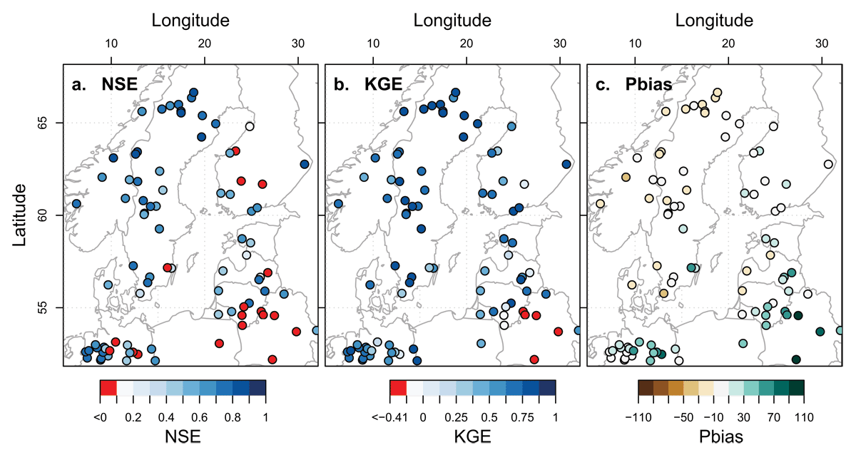
Figure 4
Evaluation of NSE, KGE and Pbias for the E-HYPE model for independent validation stations around the Baltic Sea and the Kattegat and Skagerak regions.
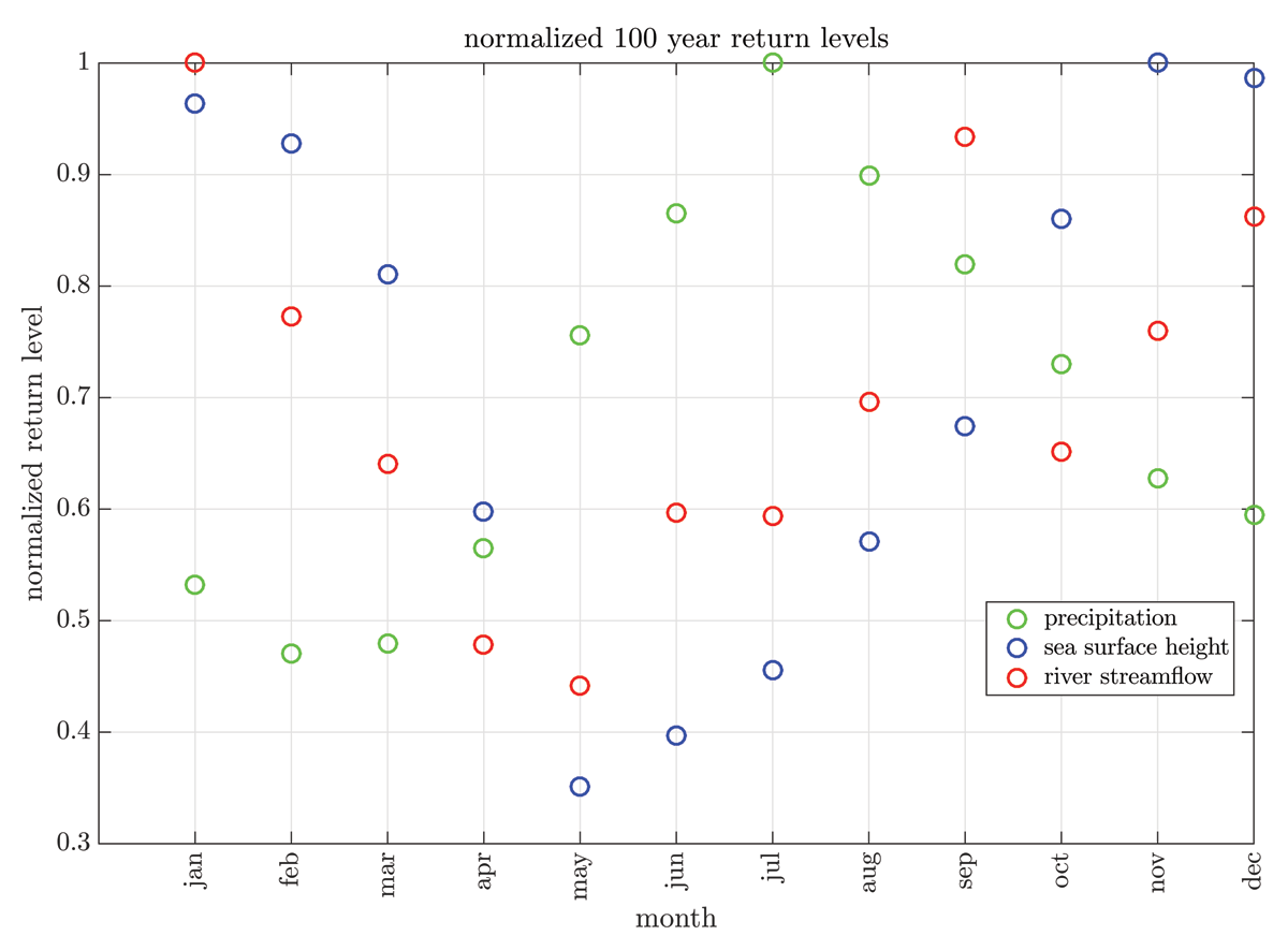
Figure 5
Normalized 100-year return level for different months. These return levels are calculated from linearly detrended time series where data from all RCPs as well as the historical simulations have been concatenated.
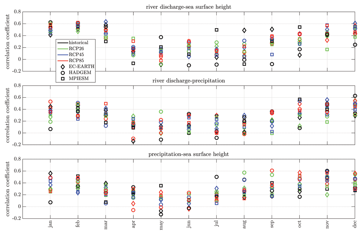
Figure 6
Correlations between annual maxima of the different hazards for different months. Each marker codes for a different global climate model that has been downscaled, while the colours code for different scenarios.
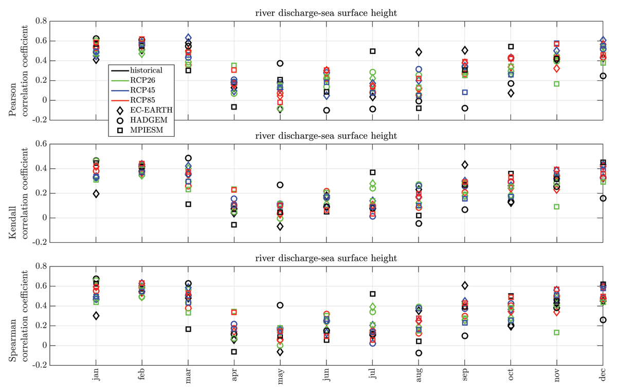
Figure 7
Pearson, Kendall and Spearman correlation coefficients between annual maxima of sea surface height and river discharge for different months. Each marker codes for a different global climate model that has been downscaled, while the colours code for different scenarios.
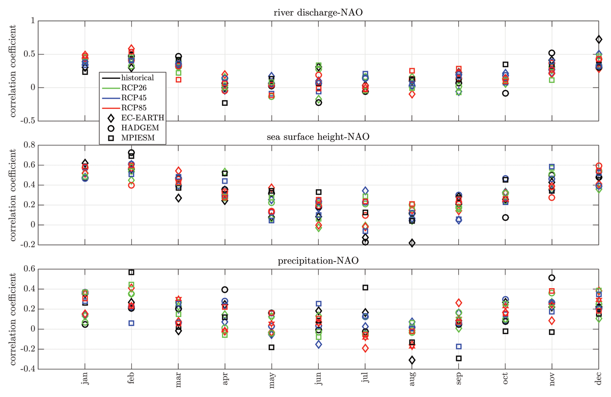
Figure 8
Same as 6, but for correlations between the hazards and the NAO.
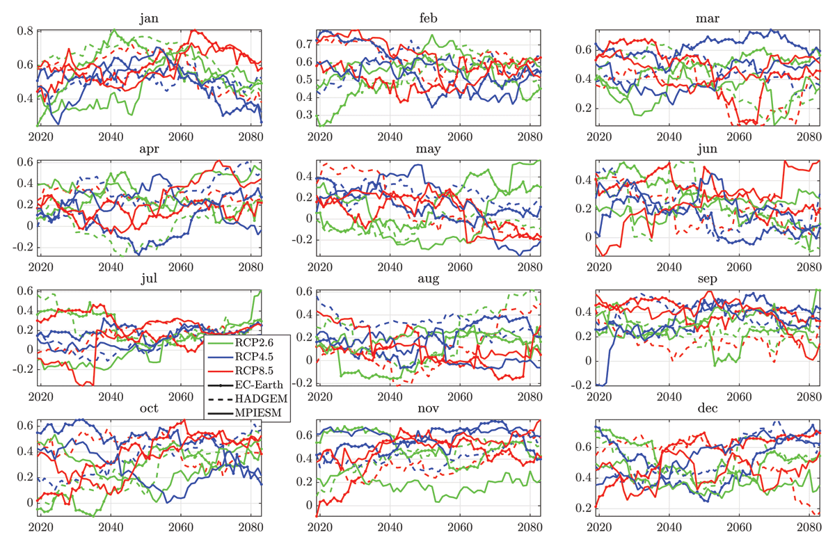
Figure 9
Running correlation coefficient calculated from 30-year periods between the annual maximum river streamflow and annual maximum sea surface height for different months.
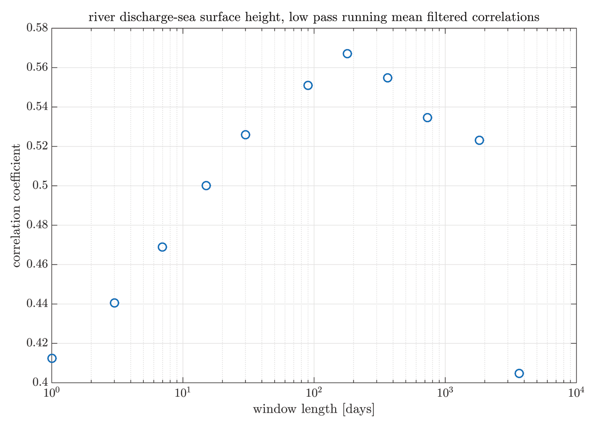
Figure 10
Correlation coefficient between low pass filtered daily mean river streamflow and sea surface height as a function of filter length. The filter used is a running mean.
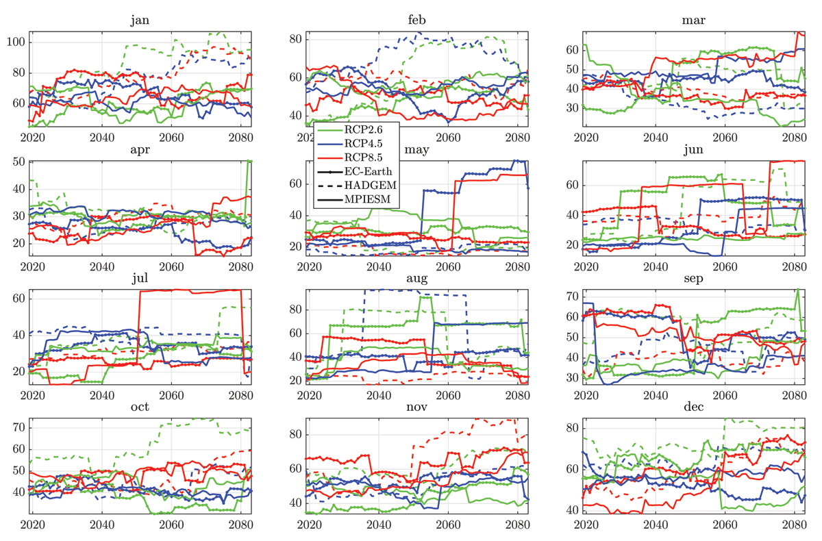
Figure 11
Running standard deviation calculated from 30 year periods of the annual maxima river streamflow for different months.
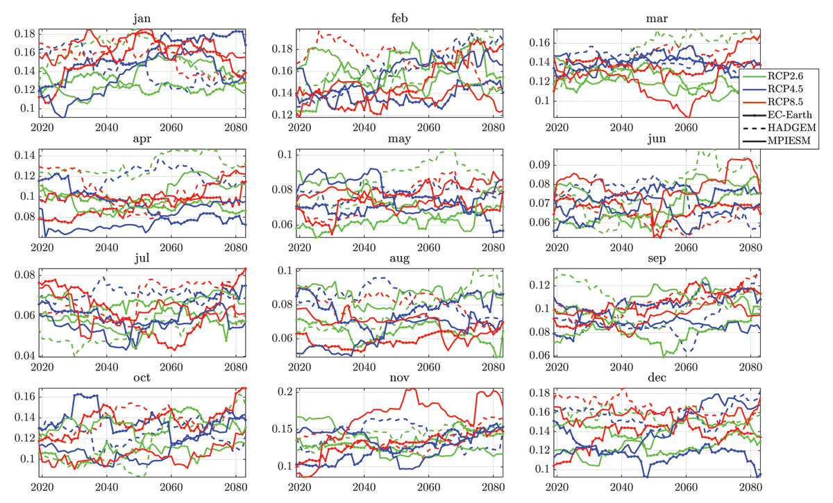
Figure 12
Same as Figure 11 but for sea surface height.
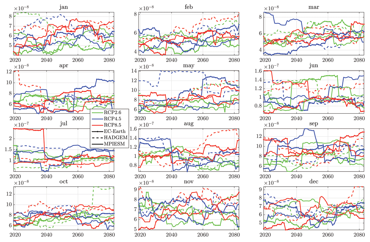
Figure 13
Same as Figure 11 but for precipitation.
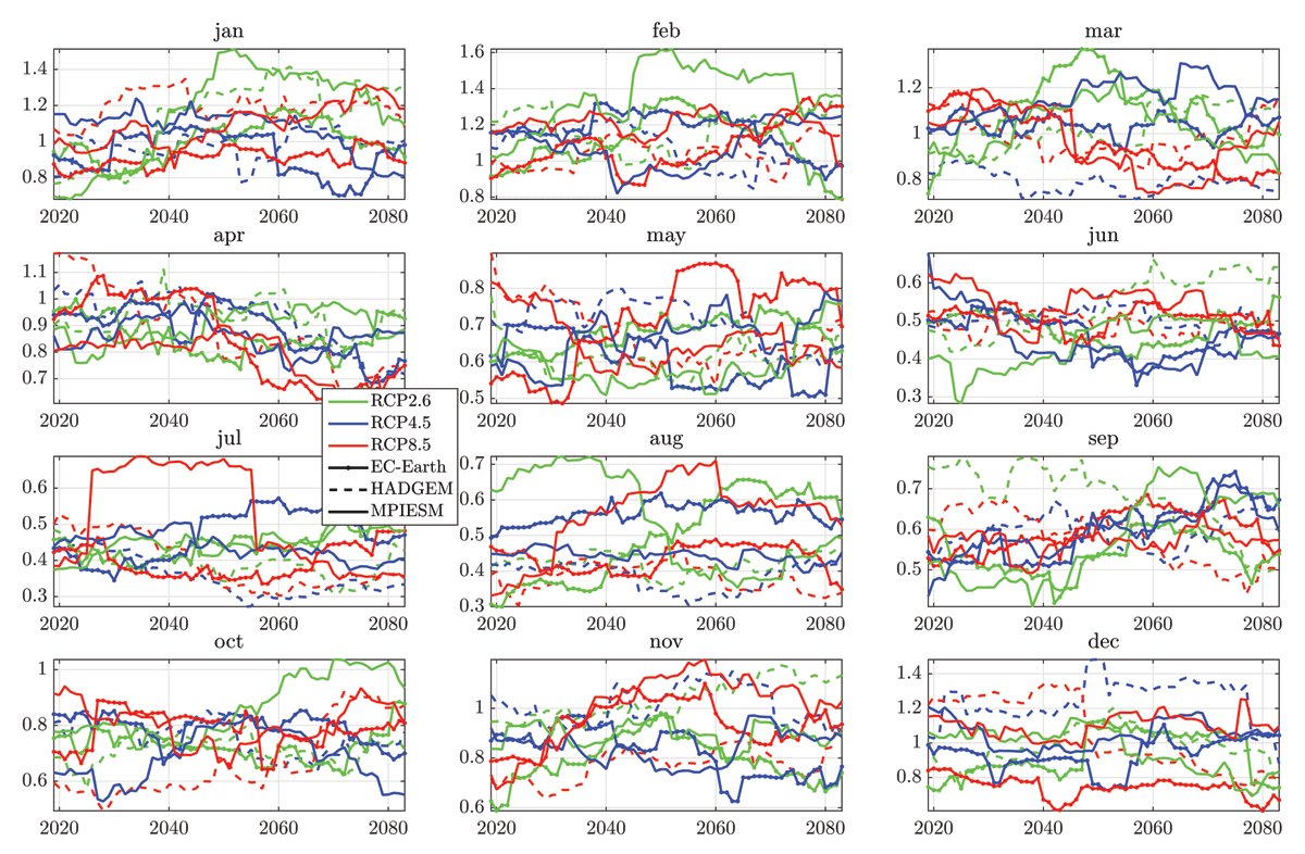
Figure 14
Same as Figure 11 but for the NAO.
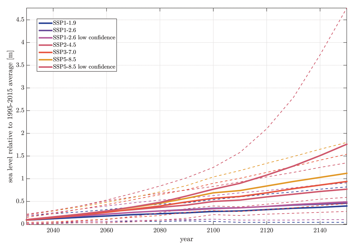
Figure 15
Mean sea level projections for Halmstad under different SSP-radiative forcing combinations. Thick lines show median projection and dotted lines likely ranges. Projections are based on Fox-Kemper et al. (2021), but the post-glacial land uplift estimates have been updated with more accurate data from Lantmäteriet (Vestøl et al., 2019).