
1 Introduction
The frequency and intensity of flooding, and thereby its cost to society, is projected to increase in the current century owing to climate change, especially in coastal areas. In Europe, coastal flooding has been projected to become orders of magnitude more expensive towards the end of the century than it is today, unless current large scale coastal defences are upgraded and new ones constructed in vulnerable areas (Vousdoukas et al., 2018). Coastal locations are more exposed to flooding than inland locations given that they can be flooded both from the ocean and from extreme rainfall (pluvial flood). If a location also happens to be close to a river then that constitutes another flood risk (fluvial flooding). Traditionally, these different flood hazards have almost always been evaluated separately. In fact, they have been the subject of study of different scientific disciplines. Coastal flooding has been studied primarily by oceanographers and coastal engineers, while fluvial and pluvial flooding have been studied primarily by hydrologists and meteorologists.
A multidisciplinary approach thus appears to be a reasonable starting point when studying compound flooding. The project Hydrohazards, where the research described in this article was conducted, is consequently populated with scientists representing a variety of disciplines, including oceanographers, coastal engineers, hydrologists, meteorologists, geographers, and social scientists. An earlier outcome of the Hydrohazards project was a nation-scale analysis of multiple water related hazards in Sweden. More on the project and its outcomes can be found through (Hydrohazards Research Team, 2024). Among the findings was that the Swedish west coast stands out as one of the few areas in Sweden, where fluvial and coastal flooding have similar seasonality. In contrast to most parts of the county, where spring floods typically occur significantly later in the year than the most extreme sea levels. Leveraging these insights, we focus on Halmstad municipality, located on the west coast of the country, to delve deeper into the analysis of compound flooding.
One may view compound flooding as the joint action of two or more random variables, where each variable represents a hazard. In the Methods sections it is shown that the joint flooding risk depends on the variance of the individual variables and the correlation between them. Our primary goal in this investigation is therefore to quantify the correlation, standard deviation, and means for sea level, precipitation and river streamflow extremes. Moreover, we will quantify them not only under current conditions, but also in an ensemble of climate change projections. A further important objective is to understand what causes co-variability between precipitation, river streamflow and sea level extremes. Essentially, we ask the question; under what atmospheric conditions are these hazards more likely to occur simultaneously or in quick succession?
Halmstad is situated in the Laholm Bay of the sea Kattegat (Figure 1). The tidal range in Kattegat is quite small, and Denmark to the west shelters the area from swells coming in from the North Sea. Moreover, the narrowness of the Kattegat limits the fetch and thus the potential for wind waves growth. In such a setting one might expect sea level extremes to be somewhat modest in magnitude, at least when compared locations further north along the Swedish coast, where the tidal amplitude is larger and the coast is more open. However, this is not the case. Instead, the tide gauge in Halmstad has been found to occasionally have sea level extremes that are considerably higher than in neighbouring locations (Johansson, 2018). In fact, the highest sea level ever recorded in Sweden was recorded by the Halmstad tide gauge in November 2015. The cause of this local effect is not known, but as will be shown in the Results section, some evidence suggests that it might be, at least partly, caused by wave set-up. The river running through Halmstad is called Nissan and is one of the major hydropower producing rivers in southern Sweden with several hydropower plants. It is therefore rather strongly regulated, which means that there is potential for management of the flow during flood hazards.
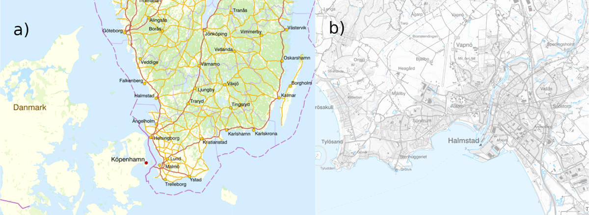
Figure 1
a) cities in southern Sweden and b) city map of Halmstad and the river Nissan that goes through the city centre. a) is taken from the Swedish land survey authority https://minkarta.lantmateriet.se/ and b) from Halmstad municipality https://karta.halmstad.se/.
Compound flooding in Halmstad was also investigated in a recent paper by Dubois et al. (2023), highlighting the importance of compound flooding in the area. Our focus is, however, on much longer time scales than those tackled by Dubois et al. (2023). Here we focus on interannual to multidecadal and even century long time scales. This naturally leads our investigation into assessing the effects of climate change on compound flooding. Long time scales and climate change was not addressed in Dubois et al. (2023). The two studies should thus be seen as complementary, having a common study area but different data, methods and scope.
Many hazards will intensify as a consequence of global warming (IPCC, 2021; Rutgersson et al., 2022). Generally speaking, much more is known about warming driven changes in the means of different variables than about changes in their variability. For example, both the total magnitude and the magnitude of individual processes contributing to current and near future mean sea level rise are rather well constrained. Moreover, how the water-carrying capacity of air increases with temperature is also well known (IPCC, 2021). However, how storminess might change in a warmer world is much more uncertain (Trenberth, Fasullo and Shepherd, 2015). The mean changes in sea level and precipitation suggest that both coastal flooding and heavy precipitation will increase in intensity and frequency in many places in a warmer future. A primary reason we know more about changes in the means than in variability of such variables is that they are predominantly thermodynamic in nature and can often be assessed directly from coarse global climate models. Changes in variability, in contrast, are often dynamically driven and inherently noisy, and ensembles of high-resolution regional climate models are often needed to assess such changes (Trenberth, Fasullo and Shepherd, 2015).
In this study, a unique ensemble of downscaled climate projections from high-resolution regional climate models is used to compute correlations between and standard deviations of river discharge, coastal sea level and precipitation. Trends in these metrics under different projections are also assessed using regional climate models as well as projections from global climate, glacier, ice sheet and glacial isostatic adjustment models, which capture processes that affect mean sea level change. Together, these data and their treatment provide the most complete assessment to date of the effects of climate change and internal variability on compound flooding in the Halmstad area.
2 Materials and Methods
2.1 Models
The model data used for this study are derived from dynamical downscalings of global coupled climate models from the coupled model intercomparison project phase 5 (CMIP5) (Taylor, Stouffer and Meehl, 2012). The atmospheric variables from the global models are further downscaled using the regional atmosphere model named RCA4 (Berg et al., 2013; Samuelsson et al., 2011). The model has a grid covering Europe and large parts of the North Atlantic, with a horizontal resolution of 25 km and 40 vertical levels. The global model is used as a boundary condition to drive the regional model.
The ocean variables are similarly dynamically downscaled using the ocean-sea ice model NEMO-Nordic (Hordoir et al., 2019; Madec and the NEMO Team, 2016). The regional ocean model covers the North Sea and the Baltic Sea with a horizontal resolution of 3.7 km and has 56 levels in the vertical. The regional ocean model is forced with downscaled atmospheric fields from the RCA4 model as its upper boundary condition. On the open boundary in the North Sea it uses a combination of monthly temperature and salinity data from the global models and hourly sea level and currents data that has been derived from the RCA4 downscalings using a machine learning approach (Hieronymus, Hieronymus and Hieronymus, 2019). NEMO-Nordic is also forced with river run-off from the E-HYPE model
The process-based hydrological model HYPE (HYdrological Predictions for the Environment; Lindström et al., 2010) simulates components of the catchment water cycle and water quality at a daily time step. The model is semi-distributed, in which a river basin may be subdivided into multiple subcatchments, which are further subdivided into hydrological response units (HRUs) based on soil type and land use classes, and is set up for a pan-European domain based on irregular polygonal catchment delineations as presented in Donnelly et al. (2016) and Hundecha et al. (2016). The E-HYPE simulations that are used as inputs to NEMO-Nordic are taken from the C3S data set (Berg et al., 2021a), where specifically the time series of river discharge from the E-HYPEcatchM00 model are used. The model simulations are driven with meteorological parameters from the accompanying data set in C3S (Berg et al., 2021b).
The complete model system, with its ocean, atmosphere and river components, is composed of standalone models forced with the same downscaled atmospheric forcing. That is, the hydrological model and the ocean model are forced using the same CMIP5 projections downscaled with the same RCA4 model. It is thus not a fully coupled system, but impacts in form of sea level, precipitation and river streamflow extremes still co-vary in a consistent manner, as all these impacts result from the same modelled atmospheric states.
Table 1 shows the climate scenarios and global climate models used in the downscalings. All scenario runs are concentration based (i.e., they are forced with atmospheric concentrations of greenhouse gases and aerosols). Our historical simulations start in 1971 and are forced with greenhouse gases and aerosols that are consistent with the observed evolution of these quantities until the year 2005. The historical simulations that were ran with global models in CMIP5 actually start in 1850, but only the period from 1971 has been downscaled, which is why our historical simulations start in 1971. The future scenarios start in year 2006, and range from low concentrations under RCP2.6 to very high concentrations under RCP8.5, while RCP4.5 is a middle of the road scenario. In terms of global mean surface temperature (GMST) increase at the end of the century compared the preindustrial; RCP2.6 gives 1.6°C, RCP4.5 gives 2.4°C and RCP8.5 gives 4.3°C (IPCC, 2013). These values refer to ensemble medians for the whole CMIP5 ensemble. GMST is, however, an emergent property of climate models so values differ between models.
Table 1
Table of downscaled global coupled models and emission scenarios. The downscaled historical simulations are not the full CMIP5 historical period. Instead they start in the year 1971. All historical simulations, however, end in the year 2005. The RCP scenarios all start in 2006 and end in 2100.
| HISTORICAL | RCP2.6 | RCP4.5 | RCP8.5 | |
|---|---|---|---|---|
| MPI-ESM-LR | X | X | X | X |
| EC-EARTH | X | X | X | X |
| HadGEM2-ES | X | X | X | X |
The RCP scenarios have not been assigned probabilities of occurrence by their makers, but some work using integrated assessment models (IAMs) has been aiming to assign such probabilities. Using information about fossil fuel resource availability, economic modelling and assuming current policies; Capellán-Pérez et al. (2016) and Huard et al. (2022) both found RCP4.5 to be the most likely scenario for the current century. The probability of having emissions as high as RCP8.5 decreased with time and reached zero in several of the IAMs probed by Huard et al. (2022) toward the end of the current century. Similarly, both Capellán-Pérez et al. (2016) and Huard et al. (2022) found the probability of having emission as low as those in RCP2.6 to be very low under current policies toward the end of the century. To sum up, future emission trajectories remain highly uncertain, but at least under current policies RCP4.5 appears to be the most likely pathway out of the three probed here.
2.2 Observations and validation
The model validation is done using daily means. This is partly because it is the available temporal resolution of the river flow data. Modelled and observed sea levels, meanwhile, are available with hourly frequency. However, since our interest is in multiple extremes, it is the possibility of these hazards to interact with each other that is our primary interest. Since the river Nissan is regulated, it is possible to, to some extent, prevent short-duration sea level extremes from coinciding with peak river discharge. Moreover, given that our focus is on long time scales, trends and interannual variability, daily means appears as a good resolution choice.
Figure 2 shows a quantile-quantile plot of daily mean sea level from our three modelled historical simulations plotted against sea level observations collected at Halmstad harbour between 2009 and 2022. The model shows a considerable underestimation of the sea level variability compared to the observations. Multiple reasons may help explain the bias. The atmospheric model very likely underestimates the surface winds, which is the primary driver of sea level variability in the area (Hieronymus, Hieronymus and Arneborg, 2017). Moreover, it is not just the wind at the time of a particular storm that is important, but also the wind the weeks and months before as it sets a baseline from which the storm surge acts. Such preconditioning has a considerable influence on sea level extremes inside the Danish Straits just to the south of our location in the semi-enclosed Baltic Sea (Andrée et al., 2023; Bellinghausen et al., 2023; Hieronymus and Hieronymus, 2021), and could potentially be important also in the Kattegat. However, it has been demonstrated that the modelling system performs much better in the Baltic Sea than on the Swedish west coast (Dieterich et al., 2019; Hieronymus, Hieronymus and Arneborg, 2017), even though the wind is underestimated over the Baltic Sea as well, suggesting that lack of preconditioning is unlikely to be a primary cause of our bias. The sea level dynamics are much more constrained by basin geometry in the semi-enclosed Baltic Sea than on the more open Swedish west coast, making the latter case harder to model. Complex basin geometry, poorly resolved by our model, is thus also likely contributing to the underestimation of sea level variability. A two-way nesting scheme giving higher resolution locally could be a way forward (Andrée et al., 2023). However, for Halmstad, there is also another potential reason for the underestimation of the modelled sea level variability. That is, the presence of a local effect that occasionally raises the sea level in Halmstad way beyond what is seen at neighbouring stations that otherwise have very similar sea level variations.
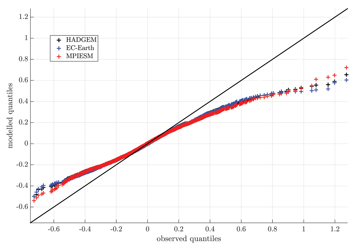
Figure 2
Quantile-quantile plot of sea level observations and modelled sea levels in our three historical simulations, see Tab. 1. All sea levels are daily means. The black line is one to one.
Figure 3 shows some sea level and wave parameters in Halmstad and at neighbouring tide gauges in Ringhals to the north and Viken to the south, during the hours when the sea level in Halmstad exceeds 1 m above the mean. The 1 m threshold is of course rather arbitrary, but the choice of threshold is not important. It merely serves the purpose of demonstrating that on some, but not all, occasions when sea levels in the area are very high they are much higher in Halmstad than in neighbouring locations. The hourly sea level measurements in Halmstad for the period 2009–2022 contain in excess of 150 observations that exceed 1 m above the mean. For a large-scale storm surge one would expect similar sea levels to be reached at these neighbouring stations. The panels showing sea level difference show that this is generally the case. However, we see at least three peaks at around t = 25, 87 and 113 when sea levels in Halmstad are significantly higher than at the neighbouring gauges. It is also evident that these peaks coincide with peaks in significant wave height. Moreover, all these incidents occur when waves are coming from the southwest. In fact, the wave direction during the times when we see a large local effect are slightly more from the south than the typical wave direction during the times when sea levels are 1 m above the mean or more in Halmstad. This might be important, as it is clear from Figure 1b that waves can only enter the small bay inside the Laholm Bay where Nissan has its river mouth from the south and southwest. This small bay is also where Halmstad harbour and our tide gauge is located. Wave set-up is a change in the mean sea level at the shoreline that is due to the presence of breaking surface waves, which in contrast to short-lived swash bores (uprush of waves collapsing on a beach) can last for significant time (Longuet-Higgins and Stewart, 1963), and may thus influence the sea level measured by a tide gauge. Moreover, an investigation from the neighbouring Baltic Sea suggests that wave set-up could give rise to considerable local water level variations in some locations (Pindsoo and Soomere, 2015).
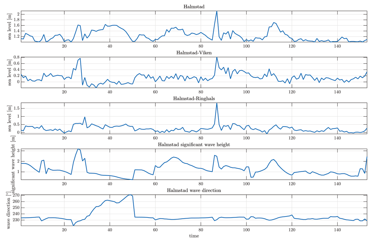
Figure 3
Sea level and wave parameters in Halmstad and at neighbouring stations during the hours in the 2009–2022 period when the sea level in Halmstad exceeded 1 m above the mean. The panels Halmstad-Viken and Halmstad-Ringhals show the sea level in Halmstad minus that in Viken and Ringhals respectively at the times when the sea level in Halmstad exceeded 1 m above the mean. The wave data comes from a reanalysis dataset produced by the Finnish Meteorological Institute (Finnish Meteorological Institute, 2023).
Other potential explanations could be wind set-up, which, in contrast to wave set-up, is part of the model’s dynamics but may be under-resolved. Another possibility is some interaction with the out-flowing river plume. We note, however, that the river discharge was not particularly high during any of these events, so such an interaction appears unlikely to be a sole or sufficient cause for the local effect. While these events present intriguing aspects, they do not constitute the main focus of our current investigation. This is primarily due to the fact that a comprehensive investigation of this phenomenon would necessitate observational data that is currently unavailable. Most prominently, one would need more tide gauges inside the Laholm Bay so the scale of the phenomena could be determined accurately.
An implication of the phenomenon’s small spatial scale and possible relation to surface wave dynamics, however, is that such events are unlikely to be well represented by the ocean model. Surface waves are not part of the model’s dynamics and a horizontal resolution of 3.7 km may well be too coarse to capture the effect. Given that wave set-up can last for significant time and have a magnitude reaching 1/4 of the wave height at the breaking line (Longuet-Higgins and Stewart, 1963; Pindsoo and Soomere, 2015), the phenomenon could explain the local effect and perhaps, at least, partly the bias seen in Figure 2. However, since that figure is based on daily means and the phenomenon is intermittent, it is likely not the sole or even primary cause of the model bias, which we believe underestimated surface winds and challenging basin geometry to be. Nevertheless, the model bias, although unfortunate, is unlikely to affect the conclusions of this study. Here our focus is on the co-variability of different hazards, which should be well captured owing to all models using the same atmospheric forcing. Moreover, the ocean model shows a high correlation to sea level observations also on the west coast when high-quality forcing is used, so the timing of extremes is generally well represented (Hordoir et al., 2019). Long-term trends in sea level are not based on the regional ocean model, but on global climate, ice sheet and glacier models (Fox-Kemper et al., 2021), so these trends are unaffected by this bias.
The E-HYPE model is calibrated on a set of calibration stations in different hydrological response classes around Europe. This approach allows parameter settings to be applied to ungauged catchments with generally good results, as evaluated with independent validation stations for each class. The model is then evaluated with separate validation stations. The performance for the validation stations around the Baltic Sea are presented in Figure 4 for the Kling-Gupta Efficiency score (KGE; Gupta et al., 2009), the Nash-Sutcliffe Efficency (NSE; Nash and Sutcliffe, 1970), and the percentage bias (Pbias) for river discharge. NSE is a measure of predictive skill of hydrological models, with values ranging from negative infinity to one, which is a perfect score. NSE = 0 is equivalent to using the mean flow as a predictor. KGE is a goodness-of-fit measure, where a value of KGE = –0.41 has a similar interpretation as NSE = 0 (Knoben et al., 2019). The model is here evaluated for the catchments with validation stations that contribute to the region of the ocean model. There was no gauge with sufficient data records for the modelled period, nor sufficiently close to the Nissan river mouth for performing a local validation. The E-HYPE model performs overall well on all three scores in this evaluation, and in an earlier evaluation for all of Europe presented in Donnelly et al. (2016) and Hundecha et al. (2020).
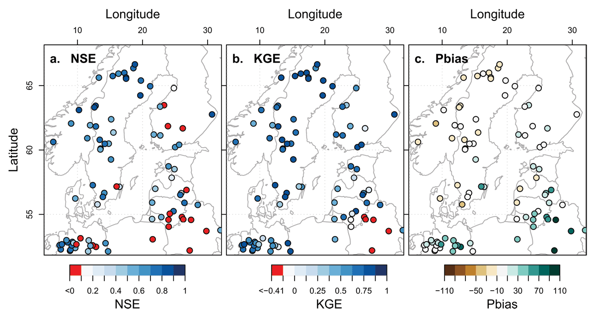
Figure 4
Evaluation of NSE, KGE and Pbias for the E-HYPE model for independent validation stations around the Baltic Sea and the Kattegat and Skagerak regions.
2.3 Methods
As discussed in the introduction, one may view compound flooding as the joint action of two or more random variables. Here we let X(t) represent time varying sea level and Y(t) time varying river discharge. Important metrics such as flooded area or property damage are then given by some functions f(X,Y). The most simple model, that might apply reasonably well to for example flooded area, would be to assume , where is the area flooded by the ocean and the area flooded by the river. In this simplified view it is easy to link the variability in the two random variables to the variability in their sum through
where σ is the standard deviation and r the Pearson correlation coefficient. The expected value, E, of the flooded area is, of course, simply
where the ≤ sign is there instead of an equal sign because the same area could be affected by both riverine and coastal flooding and should not be counted twice. The above decomposition clearly highlights that the joint flooding risk depends on the variance and magnitude of the individual variables and the correlation between them. These are therefore the main parameters investigated in the study. It should, however, be noted that our decomposition is not a full model of the dependence structure between two random variables. Such dependencies are often modelled using copulas that enables an isolation of the dependence structure in multivariate distributions (Dupuis, 2007). Some applications of copulas modelling to compound flooding is found in Bevacqua et al. (2017) and Phillips et al. (2022).
From our different downscaled climate scenarios, see Table 1. We have extracted time series of daily mean sea level, daily mean precipitation and daily mean river discharge in Halmstad. These time series are linearly detrended to remove long-term trends. This is done to study the co-variance of extremes, while trends are treated separately. Extremes are studied using time series of daily maxima for each year and calendar month extracted from our different model projections. The reason for using annual maxima time series for different months is twofold. Firstly, time series of block maxima can only converge in distribution to the Generalized Extreme Value (GEV) distribution by the Fisher-Tippett-Gnedenko theorem, so the limiting distribution is known. This extreme value version of the central limit theorem is often used with annual blocks, to infer return level curves for different hydrometeorological and oceanographic parameters. Annual maxima time series are thus a natural starting point when investigating extremes. Secondly, the division into monthly maxima gives us a way to infer the seasonality of the different extremes. Moreover, the window is short enough that multiple events occurring in the same month can be expected to lead to worse consequences than if they had been separated longer in time. That is, they can be considered as compounding events, at least in an approximate sense. From the model we also extract a normalized station based (Lisbon-Rejkavik) monthly mean North Atlantic Oscillation (NAO) index. Variability in annual sea level maxima has been connected to the NAO in observational studies on the Swedish west coast (Hieronymus and Kalén, 2020) and warrants investigation also in the model. A positive NAO typically means mild and wet winters for Sweden, whereas a negative NAO brings cold and dry air masses from the Arctic. The river flood response to these changes depends on the river, and largely on the interaction between rainfall and snow melt.
3 Results
3.1 Hazard co-variance and its trend
A fundamental prerequisite for having compounding hazards is that the hazards involved have similar seasonality. In Figure 5 we have computed the 100-year return levels for river streamflow, precipitation and sea surface height from a long annual maximum time series created by concatenating data from all our different climate projections, leading to the creation of a time series more than 1000 years long. The return levels in Figure 5 are normalized through division by the return level from the month with the highest values for the respective hazard. This gives return level values between zero and one, where one is the highest monthly return level. It is evident from the figure that river discharge and sea surface height extremes are winter intensified, while extreme precipitation occurs predominantly in summer. A natural assumption is thus that compound flooding in Halmstad is most likely to occur in winter as a consequence of co-occurring sea level and river streamflow extremes. Compound pluvial and coastal flooding will thus be our primary focus in this investigation.
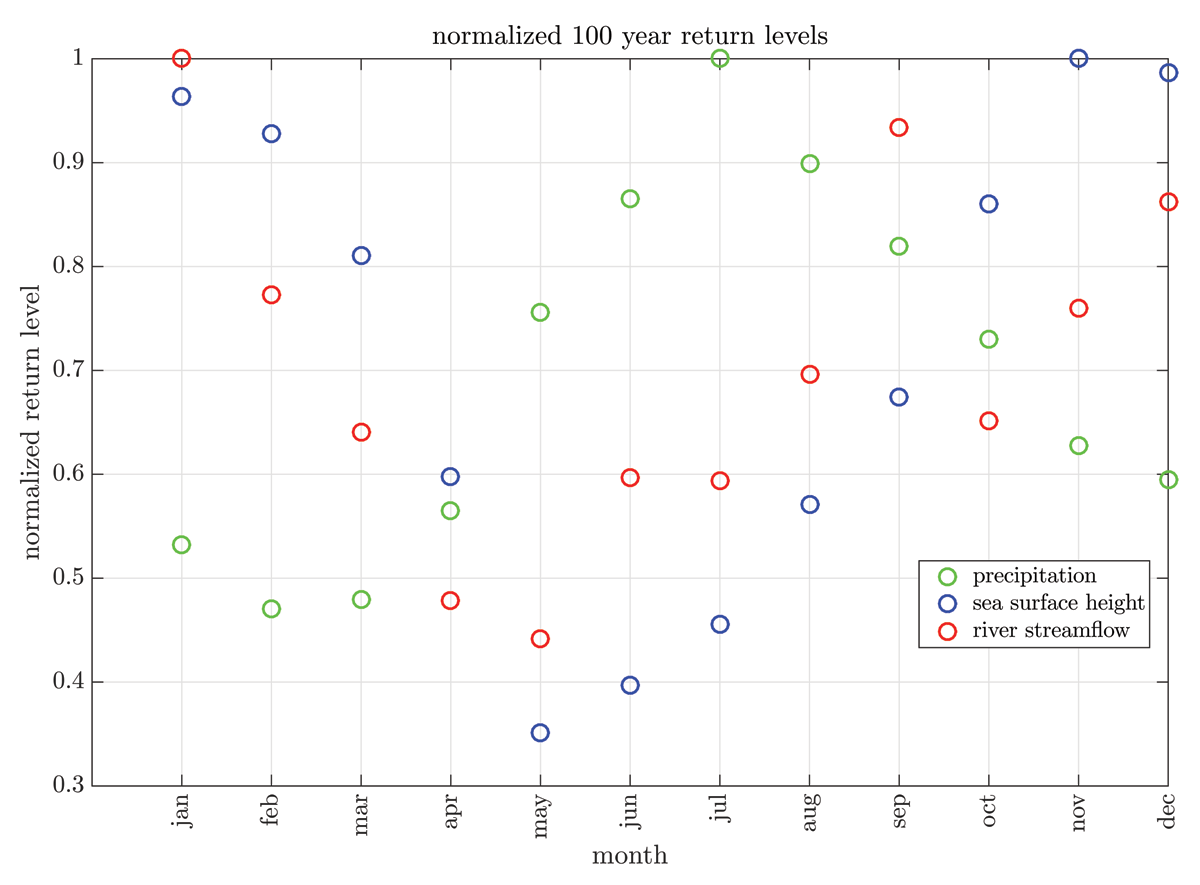
Figure 5
Normalized 100-year return level for different months. These return levels are calculated from linearly detrended time series where data from all RCPs as well as the historical simulations have been concatenated.
Equation 1 showed that the correlation coefficient between, and the standard deviations of, the different hazards are important parameters for determining compound flooding risk. In our case with three different parameters we have three different correlations to compute. River discharge to sea surface height, river discharge to precipitation and precipitation to sea surface height. These correlation coefficients for the different months are shown in Figure 6. All three panels clearly show that the annual maxima of these hazards are quite strongly correlated in winter months and uncorrelated in summer months, although with a considerable spread. Correlation coefficients exceeding |0.2| are significant at the 0.05 level in the longer RCP scenarios, while correlations coefficients exceeding |0.33| are significant in the shorter historical simulations. In this paper we focus primarily on Pearson correlation coefficients as those are the ones the that feature in our Equation 1. However, many studies of compound weather events instead use rank correlations that evaluate the monotonic rather than the linear relationship. In Figure 7 we show the Pearson, Kendall and Spearman correlation coefficients between annual maxima of sea surface height and river discharge. The results are qualitatively similar for all correlation coefficients, indicating that the relationship between the two variables is approximately linear.
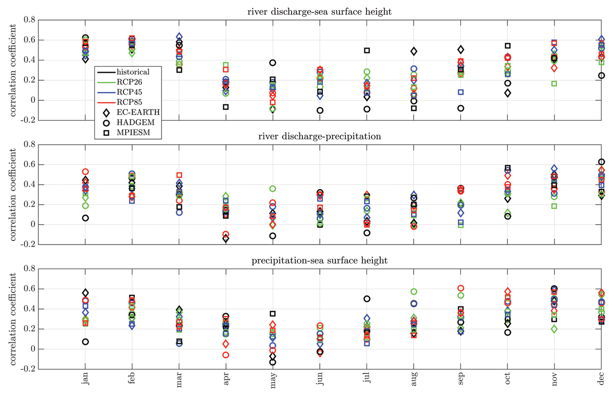
Figure 6
Correlations between annual maxima of the different hazards for different months. Each marker codes for a different global climate model that has been downscaled, while the colours code for different scenarios.
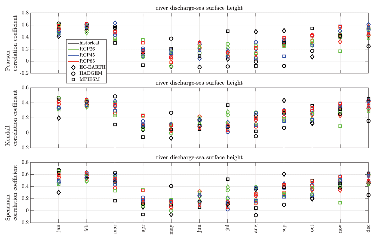
Figure 7
Pearson, Kendall and Spearman correlation coefficients between annual maxima of sea surface height and river discharge for different months. Each marker codes for a different global climate model that has been downscaled, while the colours code for different scenarios.
Low-pressure systems bringing both high precipitation and storm surges to the Swedish west coast appear as an obvious cause for the co-variability of our three hazards. A natural assumption is therefore that this co-variant interannual variability could be linked to the NAO, a connection also made for several other hazards in the Baltic Sea area by Rutgersson et al. (2022). Of particular interest for our study is that surface wave energy was recently found to correlate with the NAO in the area, making the case for compound flooding even stronger (Adell et al., 2023), as surface waves can also affect sea levels.
Correlation plots between the NAO index and our three hazards are shown in Figure 8. It is clear from the different panels that our three hazards are all correlated to the NAO in winter months. Note that the NAO index here derived is based on monthly means rather than monthly maxima (as in the hazard time series). This choice is made because we expect a connection between the atmospheric mean state and the prevalence of low-pressure systems, rather than a direct connection between extreme NAO values and extreme hazards at the site. The correlation persists, however, but is somewhat weaker if a block maxima of the NAO is used (not shown). Also noteworthy is that there seems to be no consistent difference between the scenarios or GCMs in terms of the strength of the correlations.
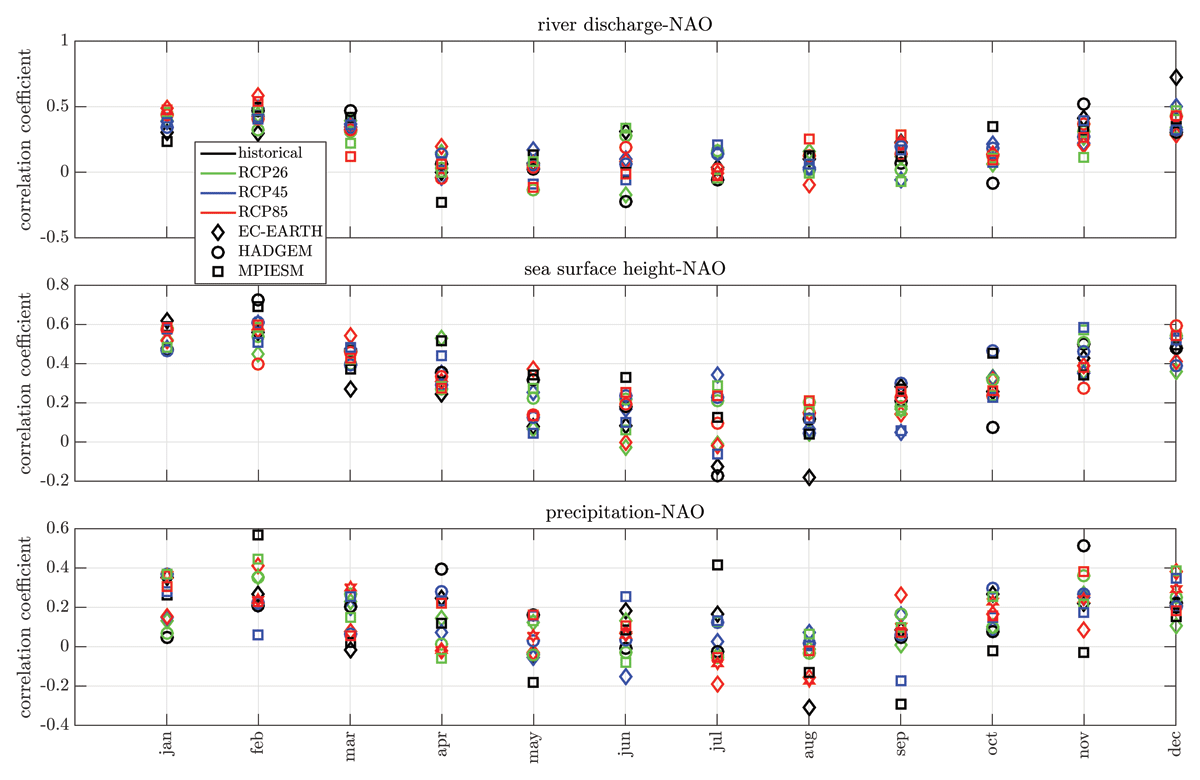
Figure 8
Same as 6, but for correlations between the hazards and the NAO.
To investigate further, we calculated the running correlation coefficient between the different hazards over 30 years periods for all months. That is, correlation coefficients are calculated for sliding 30 year periods, like a moving average but for the correlation coefficient. Figure 9 shows the result for the correlation between river discharge and sea surface height. Correlation coefficients exceeding |0.36| are significant at the 0.05 level for these 30-year period data slices. The correlation coefficients between the other hazards show similar behaviour (not shown). In all cases it is evident that the natural variability dwarfs potential warming driven trends in the correlation coefficients. A very large ensemble would be needed to get a good enough signal to noise ratio, so that a trend could be reliably estimated in the presence of this considerable natural variability. Consequently, a useful first approximation is to take these correlations to be independent of climate scenarios.
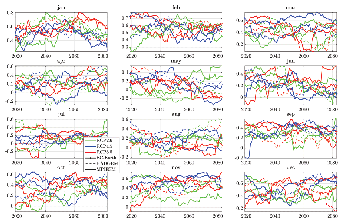
Figure 9
Running correlation coefficient calculated from 30-year periods between the annual maximum river streamflow and annual maximum sea surface height for different months.
The correlations computed from the annual maxima time series indicate coherent interannual variability between our different hazards. Next we consider the strength of the correlation on different time scales. Figure 10 shows the correlation coefficient between the low pass filtered daily mean river streamflow and sea surface height as a function of the length of the filter window. It is clear from the figure that the highest correlations are found on time scales between about 100 days and a year. These results, once again suggest an important role of interannual variability for compound flooding in the area.
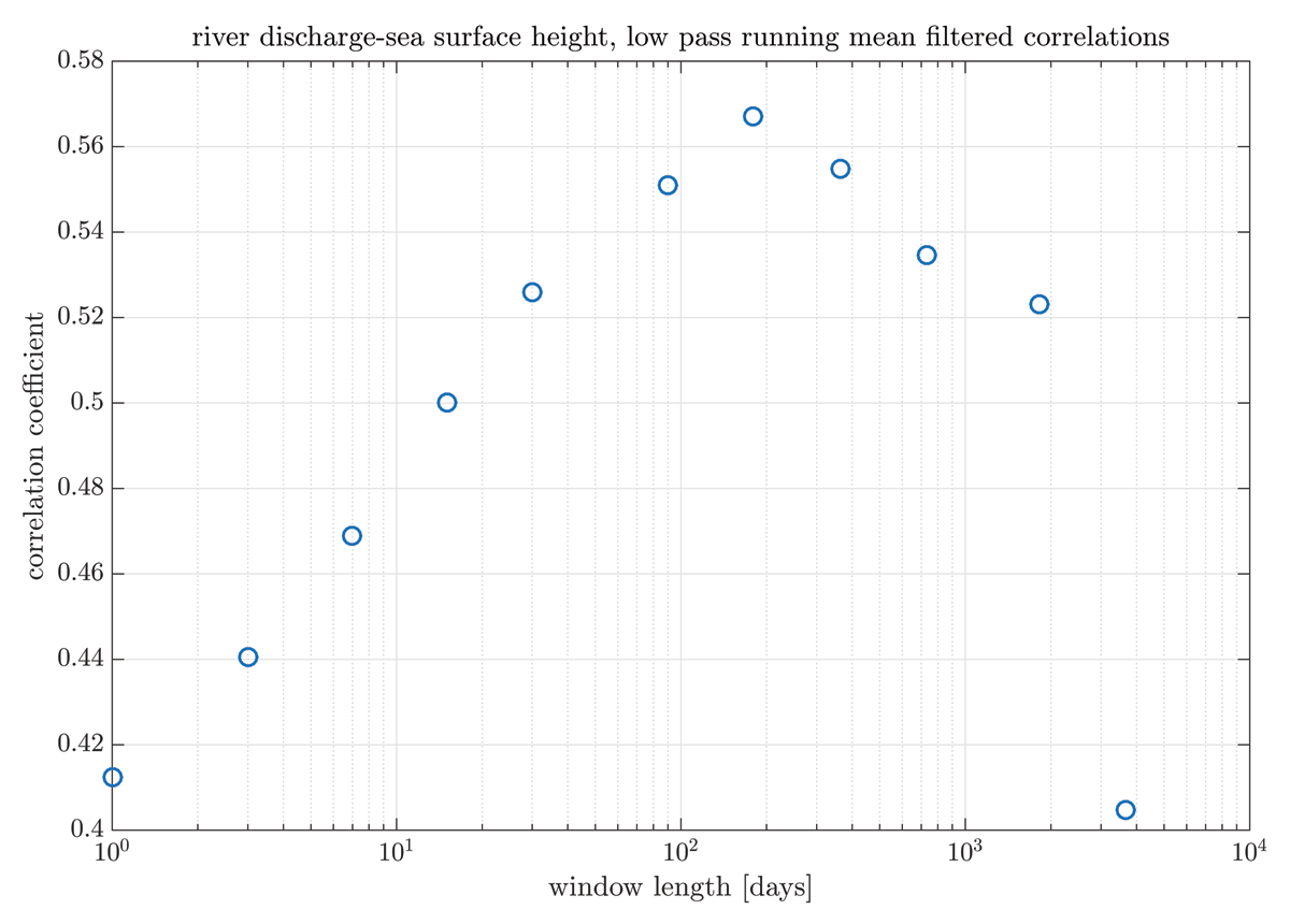
Figure 10
Correlation coefficient between low pass filtered daily mean river streamflow and sea surface height as a function of filter length. The filter used is a running mean.
Having found strong, and to a first approximation emission scenario independent, correlations between our different hazards and the NAO we proceed to investigate how the standard deviation of the different hazards and the NAO index might change in a warming world. Running standard deviations over 30-year periods are shown in Figures 11, 12, 13, 14. Given the very considerable natural variability, it is clearly not possible to discern a climate driven trend in any of these standard deviations with the amount of data we have at our disposal. However, absence of evidence does not mean evidence of absence. Thus, just as for the correlation coefficients we may conclude only that if there is a warming-driven trend, it is currently hidden within a sizeable natural variability.
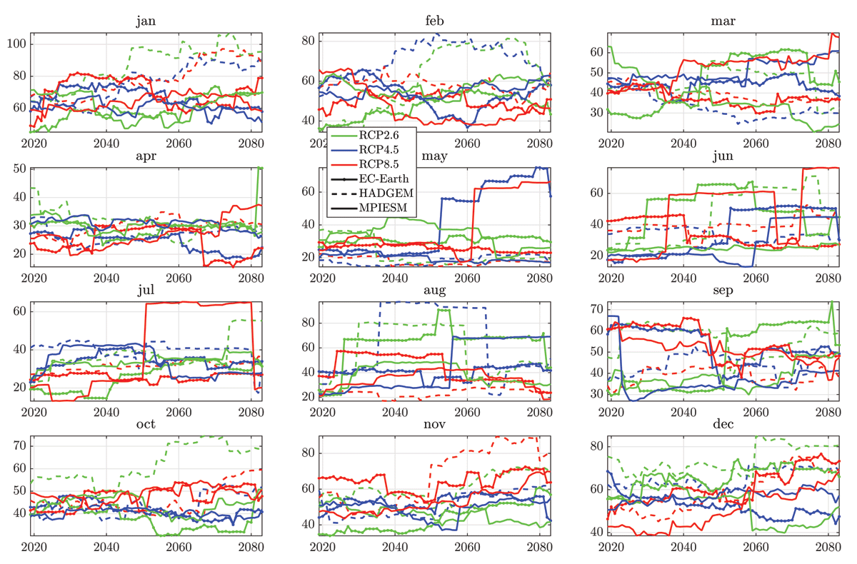
Figure 11
Running standard deviation calculated from 30 year periods of the annual maxima river streamflow for different months.
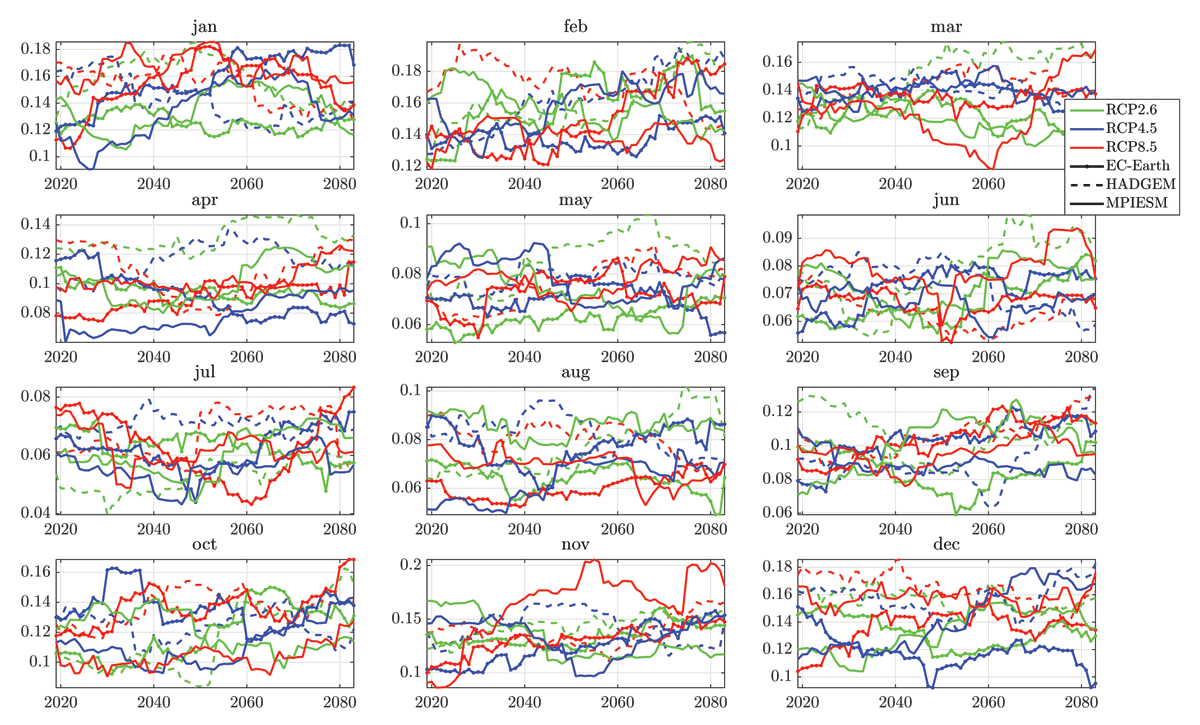
Figure 12
Same as Figure 11 but for sea surface height.
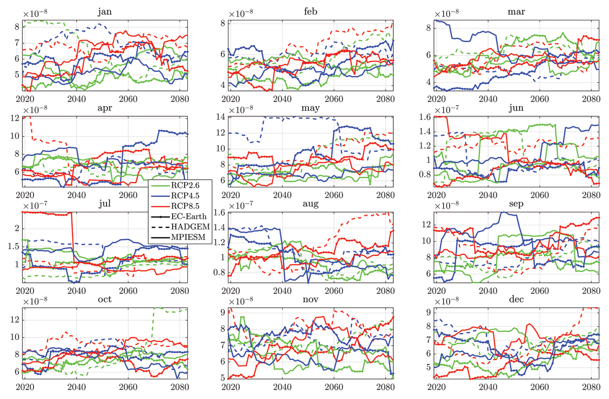
Figure 13
Same as Figure 11 but for precipitation.
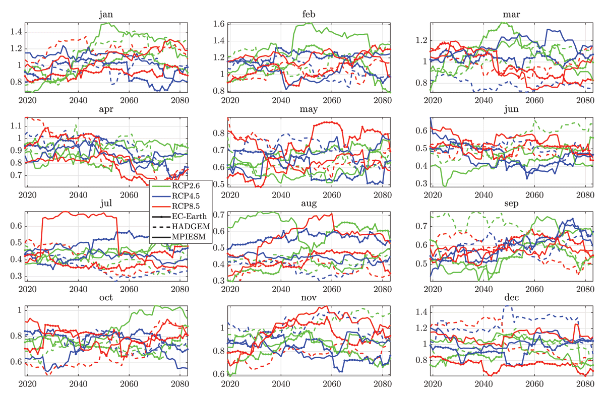
Figure 14
Same as Figure 11 but for the NAO.
As a first approximation, it thus seems fair to infer that trends in compound flooding will primarily be driven by the trends in the means of river discharge and sea level, rather than by trends in the extremes. Hieronymus and Hieronymus (2023) reached a similar conclusion for sea level extremes in the area.
3.2 Trends in individual hazards
Figure 15 shows mean sea level projections for Halmstad for a number of different shared socio-economic pathway (SSP) radiative forcing combinations based on the IPCC’s AR6 mean sea level projections but corrected with more accurate land uplift data (Fox-Kemper et al., 2021 Vestøl et al., 2019). The radiative forcing, the number after the dash given in Wm–2, is the net change in the radiative balance at the top of the atmosphere in the year 2100 compared to a pre-industrial background. A higher number implies greater warming. The mean sea level, in contrast, to the standard deviation of the daily mean sea level shows a very distinct trend under all scenarios. Coastal flood risk simulations from a number of locations around the Swedish coast have shown that flood risk is driven by the risk of high extremes in the next few decades, and by mean sea level rise in a longer perspective (Hieronymus, 2021; Hieronymus and Kalén, 2022; Hieronymus, 2023). The same is true in Halmstad, where it is clear that the land uplift of about 2 mm per year is not enough to offset significant relative sea level rise even under the very low emission scenario SSP1-1.9.
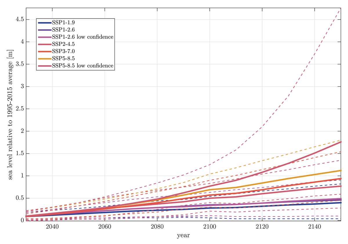
Figure 15
Mean sea level projections for Halmstad under different SSP-radiative forcing combinations. Thick lines show median projection and dotted lines likely ranges. Projections are based on Fox-Kemper et al. (2021), but the post-glacial land uplift estimates have been updated with more accurate data from Lantmäteriet (Vestøl et al., 2019).
On the other end of the spectrum we have the very high emission scenario SSP5-8.5 and its alternative projection SSP5-8.5 low confidence. In the latter, the sea level contributions from Antarctica and Greenland that are usually taken from large model intercomparison programs are instead taken from some of the highest estimates in the published scientific literature (Bamber et al., 2019; DeConto et al., 2021). In these two unlikely scenarios (Hausfather and Peters, 2020), the projected mean sea level rise toward the end of the century, is so large that it may exceed even the largest daily sea levels in the observations. In all emission scenarios, it is extremely likely that sea levels far outside of the historical range will be seen in the current century. Moreover, while the SSP5-8.5 projections represent improbable high emissions, having mean sea level rise in the meters is expected also for much lower warming scenarios albeit significantly later (Fox-Kemper et al., 2021). Therefore, when considering coastal flooding, whether as a single or multiple hazard, the most concerning trend is evidently mean sea level rise.
River discharge is affected by the competing processes of a general increase in precipitation and the increasingly intense evapotranspiration driven by temperature. The mean river discharge from Nissan shows clear evidence of increases in winter (January and February), and decreases in late spring (April and May) toward the end of the century. The median ensemble changes are rather weak for RCP2.6 (10 to 20% in January/February, and –20% in April/May), but rather strong in RCP8.5 (55 to 60% in January/February, and –35 to 45% in April/May). The annual maximum discharge shows no significant increase for RCP2.6, but some increase of 7% in RCP4.5 and a strong increase of 22% for RCP8.5, at the end of the century.
4 Conclusions
This study investigated compound flooding in Halmstad using a very comprehensive dataset of regional climate projections including hydrological, meteorological and oceanographic variables. We find river discharge and sea level extremes to have very similar seasonality, with peaks during the cold part of the year and low values in the summer. The seasonality of precipitation is more or less the opposite. From a Swedish perspective the seasonality of the river discharge stands out. Most rivers have a later peak, a defined spring flood driven by snow snowmelt. In contrast, in Halmstad we observe an earlier peak that coincides with peak storm surge activity. This makes Halmstad and other locations on the Swedish west coast potential hotspots for compound flooding.
The annual maxima for different months is found to correlate with each other and the NAO index for all three hazards during winter and autumn months. This is a clear sign of a co-variant interannual variability that one might also expect both from theory and earlier studies (Hieronymus and Kalén, 2020). It is also evident from Equation 1 that the positive correlation increases the variance of a compound flooding variable, and thus elevates the flood risk over what would be expected from un- or anticorrelated hazards.
The co-variance between the different hazards and the NAO index is potentially also important from a risk management and preparedness perspective. Seasonal forecasts from at least some models show a degree of skill on predicting the NAO (Feng et al., 2021; Wang et al., 2017). It seems not too far-fetched to claim that such information could be used together with already available short-range forecasts for the different hazards to improve the river regulation and in general the preparedness for flooding.
Trends in correlation and standard deviations were found to be dominated by natural variability in our projections, while the means of sea level, river discharge and precipitation all show considerable trends owing to anthropogenic climate change. To first order it thus seems reasonable to expect trends in the means to be driving the increased risk for compound hazards in a warming climate. This has also been shown for some individual hazards earlier, see, for example, Hieronymus and Kalén (2022) and Hieronymus and Hieronymus (2023). This finding is also aligned with the more general assessment by Trenberth, Fasullo and Shepherd (2015) that thermodynamically driven changes are larger and more easily detected than dynamically driven ones.
To conclude, it is evident that our three hazards present an elevated risk during high NAO years when their joint variance is elevated because of their correlation to each other. This is in line with the assessment by Dubois et al. (2023), who found that the co-variance of annual maximum river discharge and sea levels could lead to an elevated flood risk in Halmstad, compared to a situation where the two variables were independent. However, in Dubois et al. (2023), they found only significant correlations between the annual maximum river discharge and the sea level maxima in a three-day window around the river maximum. In contrast, when they looked at annual maximum sea level and river discharge in a three-day window around the sea level maximum, they found no significant correlation. Here we find using a much more extensive dataset that, in fact, the annual maxima of the two variables are significantly correlated and that the primary reason for this association is that both variables are affected similarly by the large scale atmospheric variability codified in the NAO index. Recent research has also shown surface wave amplitudes to be correlated to the NAO index in the area (Adell et al., 2023). Given that our results suggest that such waves may be an important component in the local sea level extremes, it seems evident that flood risk in the area is intimately tied to the NAO.
This paper, as well as others, give many insights into the hydrometeorological conditions, their variability, covariance and trends. What is still lacking is a better understanding of the impacts that these hazards might have. Future work should include a hydrodynamic flood model to assess the real-life impacts of flooding, including inundation mapping, to better understand the spatial distribution and severity of flood risks associated with compound flooding events in Halmstad. Moreover, the local, potentially wave-driven, sea level effect also warrants further investigation. However, gaining a more complete understanding of that phenomenon would likely require a long-term and extensive observation program.
Acknowledgements
The idea that the very extreme sea levels seen in Halmstad could be caused by wave set-up was suggested to us by Professor Tarmo Soomere. This work was done within Hydrohazards, a five-year project financed be the Swedish Civil Contingency Agency (MSB) and the Swedish Research Council for Sustainable Development (FORMAS).
FBA is an employee of UT-Battelle, LLC, under contract DE-AC05-00OR22725 with the US DOE. Accordingly, the US government retains and the publisher, by accepting the article for publication, acknowledges that the US government retains a nonexclusive, paid-up, irrevocable, worldwide license to publish or reproduce the published form of this manuscript or allow others to do so, for US Government purposes.
Competing Interests
The authors have no competing interests to declare.