
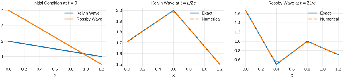
Figure 1
Initial conditions for Kelvin and Rossby waves at time that satisfy the boundary conditions (left), Kelvin wave at time (middle) and Rossby wave at time (right)
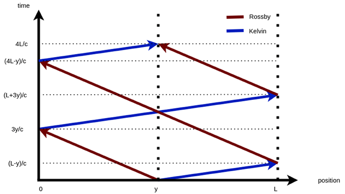
Figure 2
Kelvin and Rossby waves through characteristics.
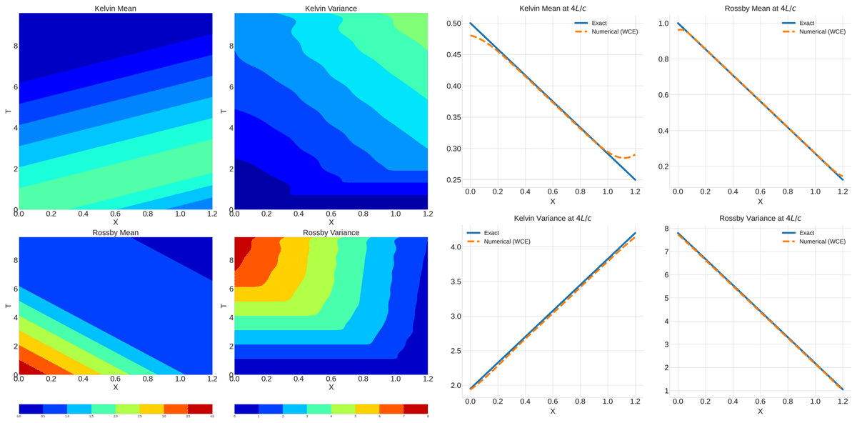
Figure 3
Mean and variance of Kelvin and Rossby waves over time (left) and at the terminal time (right).
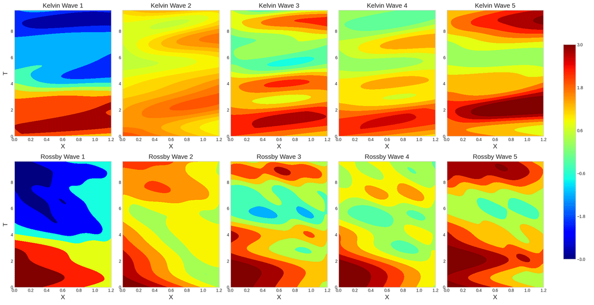
Figure 4
Random field solutions of oceanic Kelvin and Rossby waves generated using different stochastic bases.
Table 1
Gaussian random variables multiplied by the corresponding propagator coefficients for different sets.
| ξP0 | ξP1 | ξP2 | ξP3 | ξP4 | ξP5 | ξP6 | ξP7 | ξP8 | ξP9 |
|---|---|---|---|---|---|---|---|---|---|
| 1.0000 | –1.3102 | –0.0109 | 1.7551 | 1.3406 | 0.7429 | –1.2924 | 1.0150 | 0.2958 | 2.0311 |
| 1.0000 | 0.3678 | –0.5975 | –0.0969 | 0.0215 | –0.3817 | –0.7041 | 0.3456 | –0.6991 | –0.1101 |
| 1.0000 | 0.7719 | –0.6630 | 1.3424 | 0.7646 | –1.2890 | 0.1414 | –1.5045 | –1.1763 | –1.2049 |
| 1.0000 | 0.0194 | –0.2582 | 0.6723 | 0.8448 | –1.0832 | 2.0494 | 0.4994 | 1.1276 | –2.1716 |
| 1.0000 | –0.1005 | –0.1200 | –0.0088 | 0.8219 | 0.3810 | 0.1785 | 1.5316 | –0.3415 | –0.6532 |
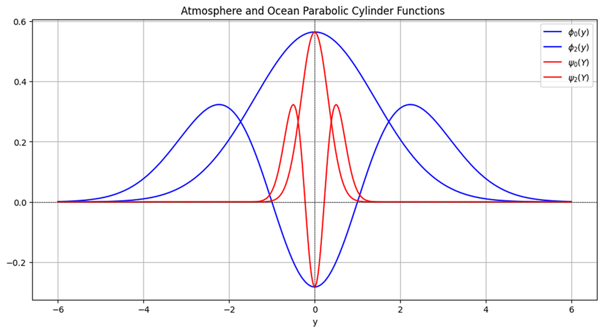
Figure 5
Meridional profiles of atmosphere () and ocean () parabolic cylinder functions and.
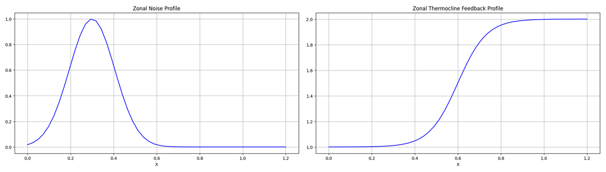
Figure 6
Zonal wind burst profile (left) and zonal thermocline feedback profile (right).
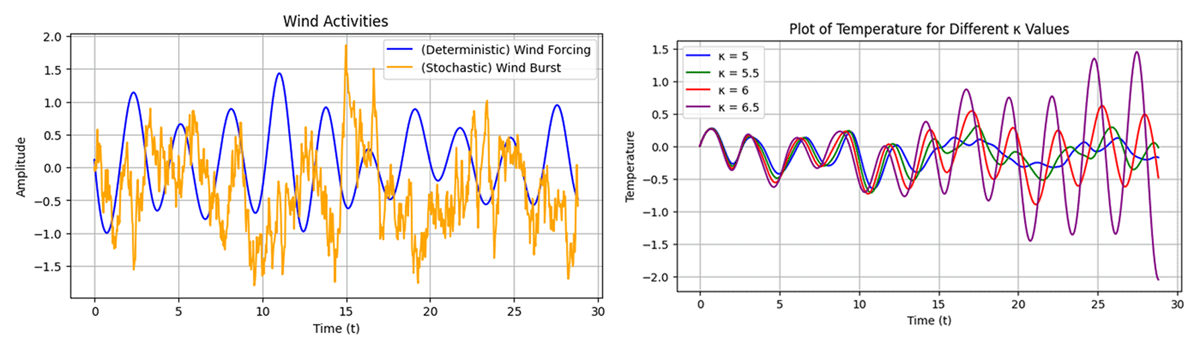
Figure 7
Deterministic and stochastic wind activities (left) and response of the SST to the different atmosphere-ocean coupling at the mid-ocean (right).
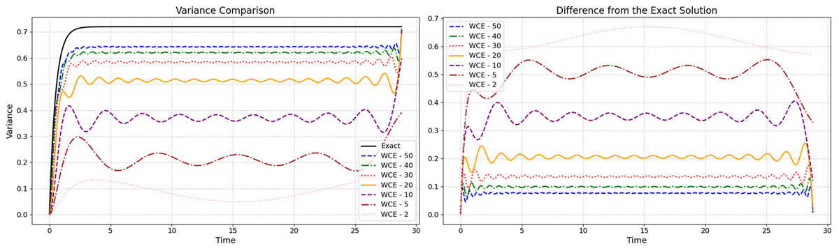
Figure 8
Variance of OU-process obtained from WCE with different number of modes , and (left) and errors relative to the exact (analytical) solution (right).
Table 2
Numerical scheme for the solution of deterministic propagators and combining with the appropriate random basis to obtain WCE solution of SPDEs.
| NUMERICAL ALGORITHM FOR WIENER CHAOS EXPANSION |
|---|
|
Table 3
Comparison of relative mean and variance errors for MC ensembles and WCE method for sea surface temperature , including computation times on a common laptop.
| RELATIVE ERROR COMPARISON: MC ENSEMBLES VS. WCE | |||
|---|---|---|---|
| METHOD | MEAN ERROR | COMPUTATION TIME | VARIANCE ERROR |
| 10 MC Ensembles | 0.3792 | 168 sec | 0.4150 |
| 50 MC Ensembles | 0.0853 | 798 sec | 0.1241 |
| 100 MC Ensembles | 0.0645 | 1627 sec | 0.1066 |
| 300 MC Ensembles | 0.0635 | 4880 sec | 0.0616 |
| 50 WCE Modes | – | 801 sec | – |
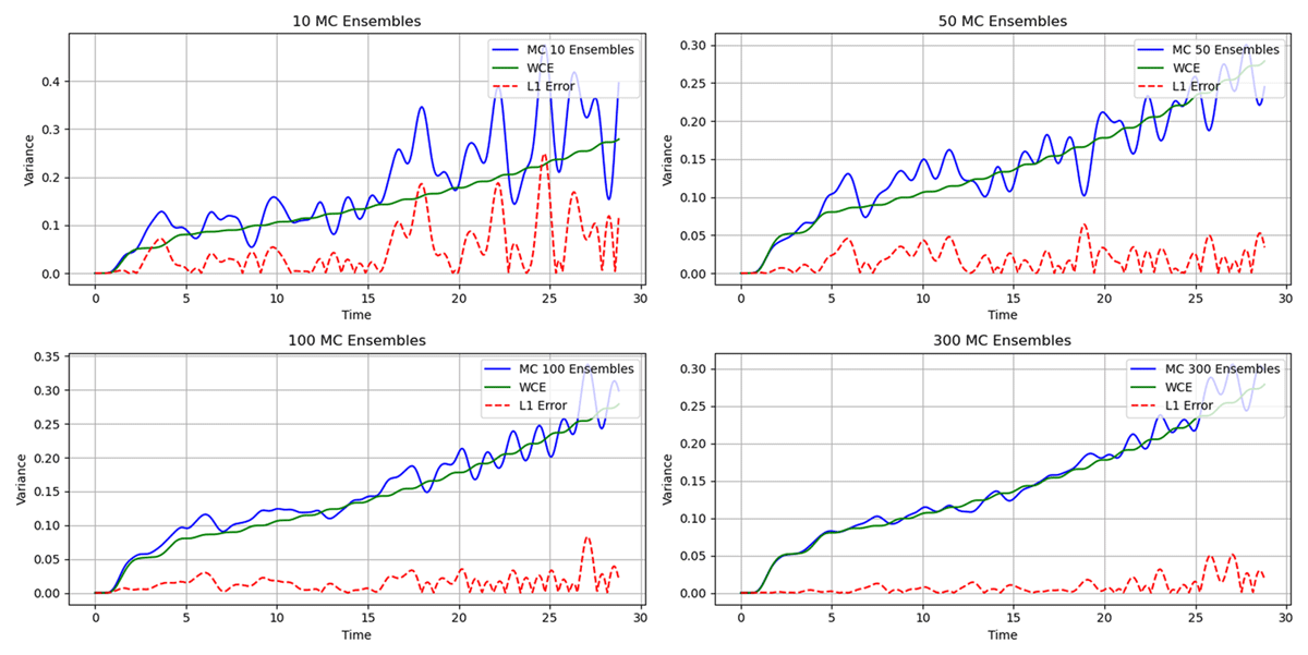
Figure 9
Comparison of WCE and MC variance results of with different number of ensembles at a fixed space point .
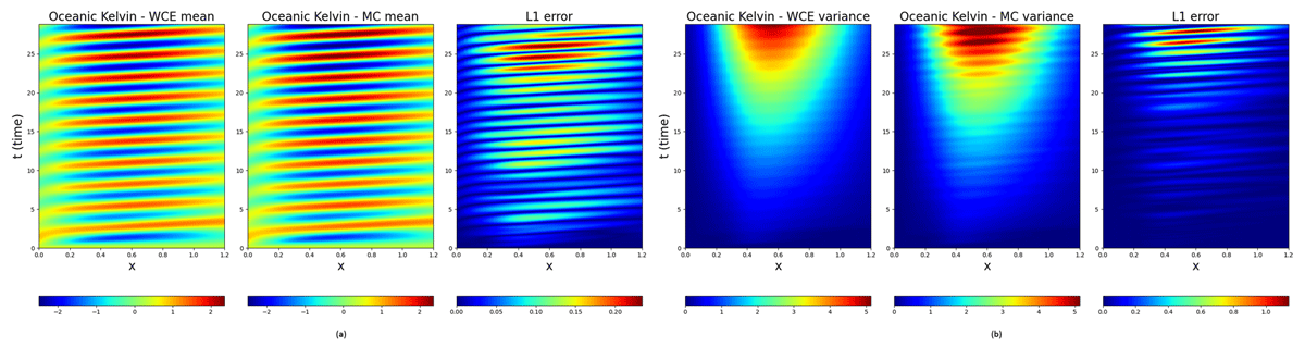
Figure 10
(a) Mean of oceanic Kelvin wave obtained from WCE (1st propagator), MC (300 ensembles), and the corresponding error. (b) Variance of oceanic Kelvin wave obtained from WCE (50 propagators), MC (300 ensembles).
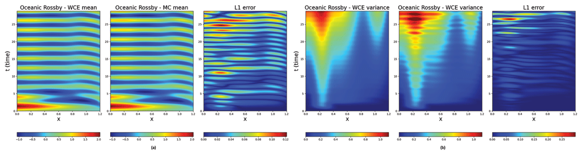
Figure 11
(a) Mean of oceanic Rossby wave obtained from WCE (1st propagator), MC (300 ensembles), and the corresponding error. (b) Variance of oceanic Rossby wave obtained from WCE (50 propagators), MC (300 ensembles).
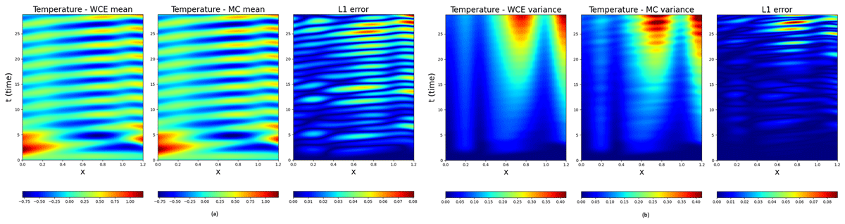
Figure 12
(a) Mean of sea surface temperature (SST) obtained from WCE (1st propagator), MC (300 ensembles), and the corresponding error. (b) Variance of sea surface temperature (SST) obtained from WCE (50 propagators), MC (300 ensembles).