
1 Introduction
The El Niño Southern Oscillation (ENSO) is a complex and recurrent climate phenomenon that originates in the tropical Pacific Ocean. It involves the interaction between the ocean and the atmosphere and has significant impacts on weather patterns around the world. First remarks of climatic anomalies at low-latitudes are based on the observations of Bjerknes in the late 1960s (Bjerknes, 1969) by recognizing the correlation between SST and equatorial atmospheric circulations. Such observations are considered as the links between El Niño and the Southern Oscillations. Along with the empirical approach, Matsuno and Gill utilized simplest and effective one-layer shallow-water models with damping and provided analytical solutions (Gill, 1980). The Matsuno-Gill model represents the atmospheric response in terms of equatorial Kelvin and Rossby waves. In addition to analytical solutions, experimental forecasts of ENSO have been made since the 1970s. Among the intermediate atmosphere-ocean coupled models derived from first principles, the Cane-Zebiak model (Zebiak and Cane, 1987) has proven influential results. The Cane-Zebiak model accurately captures the key elements of atmosphere-ocean coupled dynamics. Moreover, Neelin, Dijsktra and their co-workers proposed a comprehensive deterministic ENSO theory and analyzed system components (Dijkstra, 2006; Neelin et al., 1998).
Deterministic climate models serve as beneficial tools for gaining perspectives into the broad trends and dynamics of the Earth’s climate system. However, it is important to note that deterministic models have limitations, such as uncertainties in the initial conditions, simplifications in representing complex processes, and the deficiency to account for all relevant factors. In contrast to deterministic climate models, stochastic climate models introduce random processes to explain the internal variability and uncertainties associated with certain climate phenomena. These models are particularly useful for studying aspects of climate that exhibit inherent randomness, such as atmospheric noise, internal climate instability, and certain feedback mechanisms. Majda and co-workers recently developed a simple stochastic model that captures the main dynamics of ENSO (Chen, Majda, and Thual, 2018; Thual et al., 2016). Their approaches are based on the stochastic modeling of westerly wind bursts (WWBs) that adjust the sea temperature and shift the ocean phase. Depending on the strength of the stochastic forcing, the state is modeled as a multi-state Markov chain that switches between El Niño, non-El Niño and strong El Niño phases. Although developed models and schemes provide accurate results of ENSO, there are still several limitations for the prediction of ENSO phenomenon (Kleeman and Moore, 1997) due to the sensitivities to the stochastic forcing. Therefore, it is important to develop appropriate stochastic models, numerical schemes and effective techniques for the accurate prediction of ENSO dynamics.
In this paper, we study the effects of the stochastic perturbations on the ENSO dynamics and explore novel modeling and numerical schemes based on the Wiener chaos expansion (WCE) and compare with the Monte Carlo (MC) simulations. WCE was originally introduced by Wiener (Wiener, 1938) in 1938 and later extended by Cameron and Martin (Cameron and Martin, 1947). The idea is the explicit discretization of white noise through Fourier expansion. WCE is closely associated with proper orthogonal decomposition (POD), Karhunen-Loève (KL) decomposition, and various other spectral methods (Xiu and Karniadakis, 2002).Theoretical foundations of WCE and some important numerical applications including 1D wave equation, Burgers equations and Navier-Stokes equations can be found in (Kalpinelli, Frangos, and Yannacopoulos, 2013; Lototsky and Rozovskii, 2006; Luo, 2006).
The WCE framework offers several appealing characteristics that make it potentially well-suited for numerical computations. These include the advantageous separation of random and deterministic components of the dynamics, as well as the feasibility of the resulting approximations as probability densities in random physical systems. However, it has some limitations due to high dimensionality, nonlinearity, and approximation accuracy as broadly mentioned in (Majda and Branicki, 2012).Therefore, combining and comparing WCE with the MC approach is particularly useful for dealing with random processes whose statistical properties are not well-known.
This paper is organized as follows: In Section (2), we work on the simple ocean model driven by white noise. The problem is modeled by the oceanic Kelvin and Rossby waves coupled at the ocean boundaries with reflective boundary conditions. We first analyze the discontinuities of the homogeneous model in Section (2.1) We provide the exact solution using method of characteristics and compare with the numerical solutions obtained by using WCE in Section (2.2). After introducing background and construction of white noise and WCE in (2.3), we compare the analytical and numerical solutions in (2.4). In Section (3), we study a linear stochastic ENSO model and provide some important deterministic and stochastic modeling features. In Section (4), we apply the WCE method on the Ornstein-Uhlenbeck process with a specific dissipation and noise strength and demonstrate that the first few WCE modes can capture over 90% of the variance energy. Finally, we present a WCE-based numerical solution and discuss the results by comparing the MC-based approach for high-dimensional stochastic ENSO model in Section (4) and (5).
2 Simple Ocean Model Driven by White Noise
An essential component of ENSO modeling is the propagation of ocean waves. To analyze and test the efficiency of the proposed WCE method, we first employ the simple ocean problem modeled by the oceanic Kelvin and Rossby waves driven by white noise. The problem can be formulated as follows:
where , and represent the oceanic Kelvin and Rossby waves and Brownian motion with a constant noise strength , respectively. Therefore, the solution is the function of spatial-time variable, but also the Brownian motion. The model has reflective boundary conditions
where and are coupling coefficients at the western and eastern ocean boundaries, respectively. Initial conditions that are shown explicitly in the next section are defined as:
Kelvin and Rossby waves play significant roles in the dynamics of the ENSO in the tropical Pacific Ocean. Kelvin waves travel eastward along the equator, constrained by the Coriolis effect, which is zero at the equator. On the other hand, Rossby waves, which travel westward and are much slower than Kelvin waves, are large-scale waves generated by the Earth’s rotation and the variation of the Coriolis effect with latitude. In climate models, accurately representing these waves is essential for simulating the timing, intensity, and duration of ENSO events. These waves are also the first meridional basis projection to the originally two-dimensional PDEs- and help modulate the sea surface temperature anomalies that are central to ENSO dynamics, as discussed in more detail in Section (3).
2.1 Discontinuities of the homogeneous model
To analyze the model features, we consider the homogeneous (unforced) case of equations (1)–(3) where and . Due to the reflective boundary condition at the ocean boundaries, the model has discontinuities. We use a simple linear initial condition as shown in Figure 1. Although this initial condition may not be physical, it is one of the simplest choices that satisfy the boundary condition of the model.
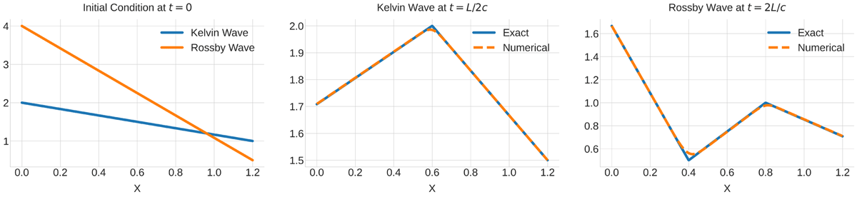
Figure 1
Initial conditions for Kelvin and Rossby waves at time that satisfy the boundary conditions (left), Kelvin wave at time (middle) and Rossby wave at time (right)
By using the method of characteristics, we observe that has a jump discontinuity at all times and . At time , the exact solution can be written as:
Similarly, has one jump discontinuity at times and and two jump discontinuities at times . We have the solution for at time as follows:
Figure 1 depicts the comparison of numerical solution and exact solution obtained from the characteristics of Kelvin wave at time and Rossby wave at time . The figures illustrate that the error between the exact and numerical solutions is remarkably small.
2.2 Mean and variance through characteristic lines
In this section, we study the exact solution of the statistical moments of the ocean problem (1)–(3). We obtain mean and variance solutions at the terminal terminal time and then compare with the numerical solutions generated from the WCE.
Figure 2 illustrates the propagation of oceanic Kelvin and Rossby waves through characteristic lines. The horizontal axis represents the position of the waves in the ocean domain, while the vertical axis indicates the reflection times at the boundaries. Waves starting their motion at the point return to the same point within one-period time, calculated as for this problem. At the boundaries, the waves transform into each other due to the reflective boundary conditions. The mean value of is while the variance is given by
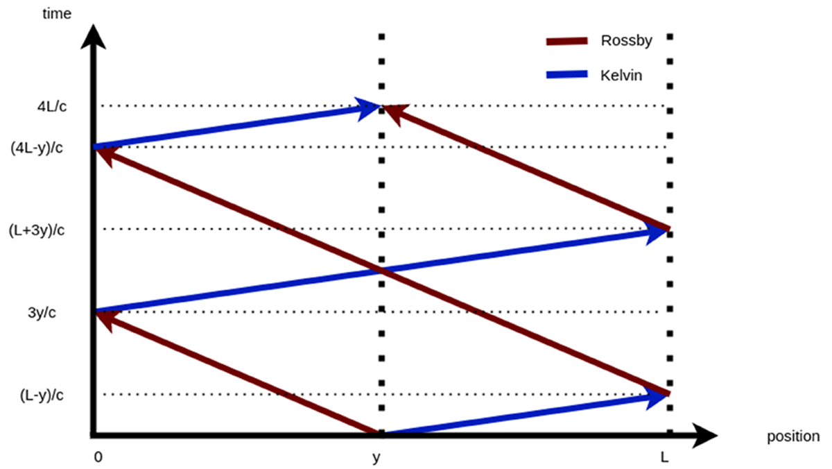
Figure 2
Kelvin and Rossby waves through characteristics.
Similarly, the mean value of is while the variance is given by
In the next section, we compare the exact solutions of the mean and variance equations (6)–(7) at the terminal time with the numerical solutions obtained from the WCE-based method.
2.3 Wiener chaos expansion
Wiener chaos expansion is a mathematical technique used in stochastic analysis to represent random variables or stochastic processes as infinite series of orthogonal polynomials. The method is particularly applied in the context of stochastic partial differential equations (SPDEs) to efficiently describe the randomness in the solution. A SPDE forced by Brownian motion has the general form
where is a (linear or nonlinear) differential operator and is a Brownian motion. The solution of SPDE (8) depends on the realization of the Brownian motion forcing. For any fixed time , assume , are a set of complete orthonormal bases in the Hilbert space . Then, Brownian motion can be constructed by using the following Fourier expansion
That can be interpreted as the projection of the white noise onto the basis function . In this paper, we use the following orthonormal basis functions of the Brownian motion:
where , in which depends on the order of truncation. In (Luo, 2006), it is shown that the expansion (9) converges in the mean square sense for all :
Thus, using a large number of basis functions results in a closer approximation to Brownian motion with reduced error. According to the Cameron and Martin theorem (Cameron and Martin, 1947), the solution can be represented by infinite series as a Fourier-Hermite series of Gaussian random variables
where are deterministic WCE coefficients (also called propagators (Lototsky, Mikulevicius, and Rozovskii, 1997; Lototsky and Rozovskii, 2006; Luo, 2006)) and are multi-variable Hermite polynomials (also known as Wick polynomials) of Gaussian random variables as
The expansion (12) particularly separates the deterministic effects from the randomness in the random field solution. Once the solutions of propagators are found by using standard numerical methods, statistical moments such as mean and variance can be calculated by using the solutions of WCE coefficients. To obtain a systematic recursive set of equations, the set of multi-indices is defined as
The set is countable and for every , only finitely many of are not equal to zero. For instance, is order index while or are the order indexes. Higher order indexes or are order and are computed for the nonlinear problems. However, it should be noted that, for the linear problems of this paper, the stochastic part is written first order Hermite polynomials . The mean and variance of the problem can be calculated by using the following propagators, respectively:
and
2.4 Comparison of theoretical and numerical results
We simulate the model until , which corresponds to one-period time where and . Figure 3 illustrates the evolution of Kelvin and Rossby wave mean and variance, calculated using Equations (15)–(16), over one-period. We compare the mean and variance results of the exact solution (as obtained in the previous section using characteristics) with those from the WCE at the terminal time and find reasonable agreement using 1-WCE mode for the mean 9-WCE modes for the variance. As the mean solution decays due to dissipation at the boundaries, the variance increases over time due to stochastic forcing. Due to discontinuities in the boundary conditions, some errors are observed in the numerical solution at the boundaries for the mean calculations.
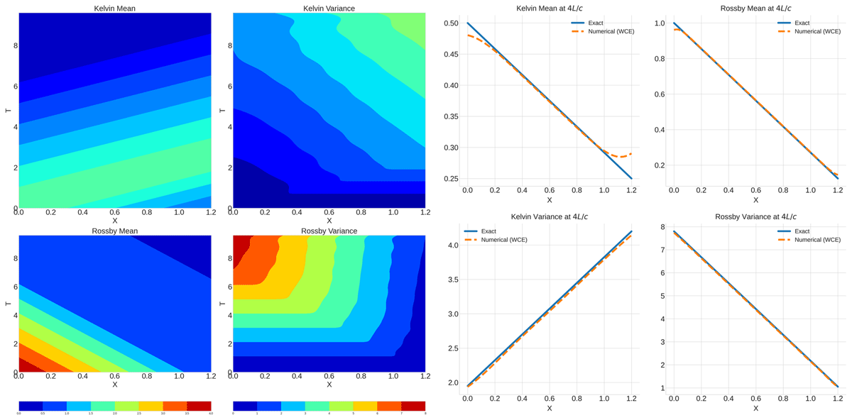
Figure 3
Mean and variance of Kelvin and Rossby waves over time (left) and at the terminal time (right).
To obtain the random solution for , we combine the deterministic propagators with the corresponding Hermite polynomials. Random numbers are generated by using the Python package numpy.random.normal with a normal distribution . Table 1 shows one set of random variables to obtain a complete random solution of model (1). After deriving the expressions for the propagators, we combine them with the corresponding random Hermite bases. Figure 4 displays five ensemble solutions of Kelvin and Rossby waves. Due to the stochastic nature of the solutions, each ensemble exhibits different wave evolution.
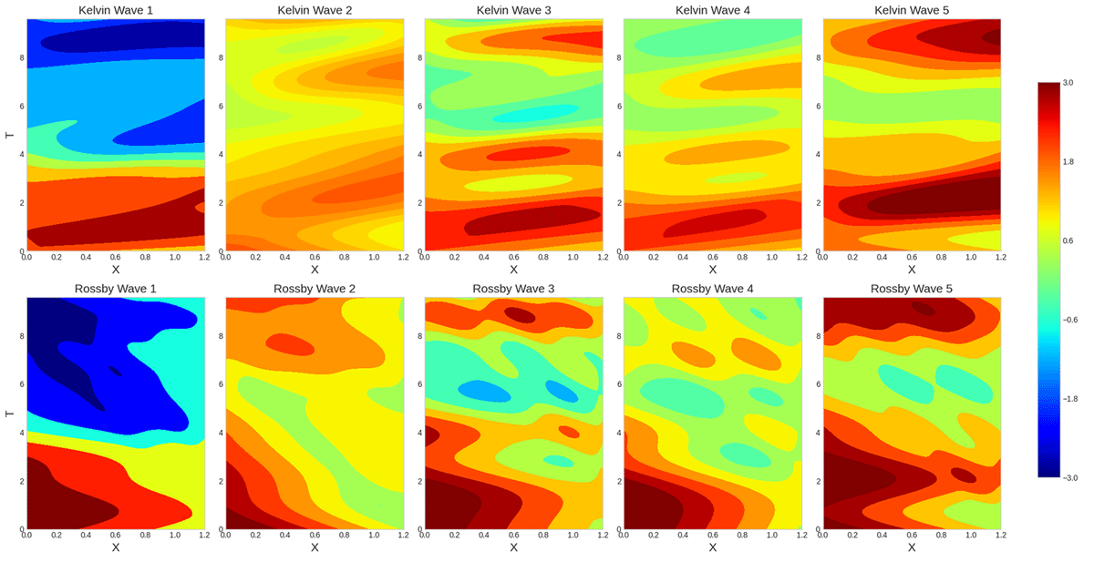
Figure 4
Random field solutions of oceanic Kelvin and Rossby waves generated using different stochastic bases.
Table 1
Gaussian random variables multiplied by the corresponding propagator coefficients for different sets.
| ξP0 | ξP1 | ξP2 | ξP3 | ξP4 | ξP5 | ξP6 | ξP7 | ξP8 | ξP9 |
|---|---|---|---|---|---|---|---|---|---|
| 1.0000 | –1.3102 | –0.0109 | 1.7551 | 1.3406 | 0.7429 | –1.2924 | 1.0150 | 0.2958 | 2.0311 |
| 1.0000 | 0.3678 | –0.5975 | –0.0969 | 0.0215 | –0.3817 | –0.7041 | 0.3456 | –0.6991 | –0.1101 |
| 1.0000 | 0.7719 | –0.6630 | 1.3424 | 0.7646 | –1.2890 | 0.1414 | –1.5045 | –1.1763 | –1.2049 |
| 1.0000 | 0.0194 | –0.2582 | 0.6723 | 0.8448 | –1.0832 | 2.0494 | 0.4994 | 1.1276 | –2.1716 |
| 1.0000 | –0.1005 | –0.1200 | –0.0088 | 0.8219 | 0.3810 | 0.1785 | 1.5316 | –0.3415 | –0.6532 |
3 Linear Coupled Stochastic ENSO Model
In this section, we utilize the linear stochastic ENSO model introduced by Majda and co-workers (Chen, Majda, and Thual, 2018; Thual et al., 2016) to show the accuracy of the WCE method for high dimensional coupled problems. The dissipative steady atmosphere model is driven by atmospheric Kelvin and Rossby waves, respectively. Additionally, a dissipative shallow water ocean model forced by atmospheric waves and stochastic wind burst is composed of oceanic Kelvin and Rossby waves. Final component of the coupled model is the sea surface temperature (SST) model that characterizes the temperature anomalies. Linear coupled PDEs in six variables can be written in differential equation form as
where the linear operator in terms of bifurcation , the wind stress coefficient
and is constant matrix, external forcing vector and noise vector are given by
We have the following boundary conditions for the atmosphere variables that are confined in the ocean domain:
where and represent the length of the equatorial belt and Pacific ocean, respectively. We have the following reflective boundary conditions for the ocean variables:
where and represent the western and eastern parts of the ocean, respectively. Initial conditions for the model can also be written as:
Atmospheric and oceanic Kelvin and Rossby waves play crucial roles in the ENSO dynamics. During an El Niño event, Kelvin waves often cause the thermocline to deepen in the central and eastern Pacific. As these waves travel eastward, they can cause an increase in SST by bringing warmer waters to the central and eastern parts of the Pacific Ocean. On the other hand, Rossby waves can modulate the influence of Kelvin waves by altering the large-scale ocean circulation patterns and can contribute to the overall variability in SST by modulating oceanic heat transport and mixing processes.
Although we consider only the one-dimensional model in this paper, after solving the system (17), one can reconstruct the two-dimensional (zonal and meridional) model using the atmospheric and oceanic parabolic cylinder functions, as illustrated in Figure 5. The first atmospheric parabolic functions read , , while the ocean parabolic functions read where (Chen, Majda, and Thual, 2018; Thual et al., 2016). The parabolic cylinder functions in the ocean and atmosphere differ due to the Rossby radius. Some important features of the ENSO model are depicted in Figures 6 and 7. Stochastic wind bursts force the ocean variables with the spatial profile notably impacting the western half of the ocean, particularly the first quarter, as shown in the Figure 6. The thermocline depth, influenced by the oceanic Kelvin wave and Rossby wave , is incorporated into the SST component through the thermocline feedback variable .
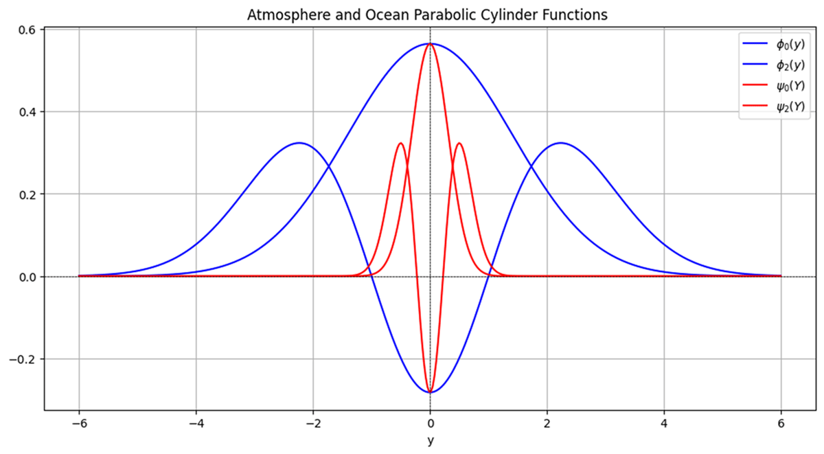
Figure 5
Meridional profiles of atmosphere () and ocean () parabolic cylinder functions and.
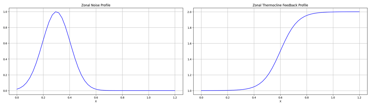
Figure 6
Zonal wind burst profile (left) and zonal thermocline feedback profile (right).
In our numerical simulations, we observe that the initial conditions of the model keep dominating the system until around time . Therefore, we simulate the model until 3-period, which is , to analyze both transient and steady states. Ocean is forced by the atmosphere in two ways : (i) deterministic forcing caused by the wind flow and and (ii) stochastic forcing created by the wind burst activities . Figure 7 depicts the time evolution of atmospheric forcing () at the mid-ocean with coupling coefficient , dissipation , noise strength and mean .
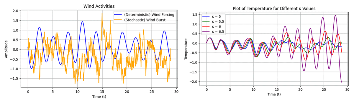
Figure 7
Deterministic and stochastic wind activities (left) and response of the SST to the different atmosphere-ocean coupling at the mid-ocean (right).
Figure 7 also depicts the response of SST at the mid-ocean to the coupling coefficient between atmosphere and ocean. As the coupling strength increases, the ocean is forced by the atmosphere with higher strength. This response grows significantly after surpassing a certain threshold value of which acts as a bifurcation parameter.
4 Results
We first apply WCE to the Ornstein-Uhlenbeck (OU) process, which models stochastic wind burst activities affecting the ocean. Figure 8 shows the variance of the OU process for different numbers of WCE modes, along with the corresponding errors relative to the exact solution. We observe that a small number of modes, such as 2, 5, and 10, fail to capture more than 50% of the variance. In contrast, after using 40 modes, the WCE variance results converge closely to the exact values. Since 50 modes capture over 90% of the variance, we can effectively use 50 modes to represent the OU variance and coupled model, achieving a satisfactory convergence to the random field solution of the problem.
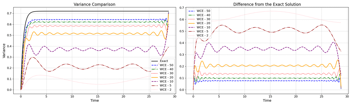
Figure 8
Variance of OU-process obtained from WCE with different number of modes , and (left) and errors relative to the exact (analytical) solution (right).
To apply WCE for the coupled high dimensional problem, we first truncate the propagator equations that can be solved by well-known numerical schemes. We use upwind finite difference schemes for the ocean and SST components and numerical integration for the atmosphere as shown in Appendix. The solutions of propagators are used to calculate the mean and variance of the model. Finally, one can construct the stochastic bases by using Gaussian random numbers and can combine them with the deterministic propagators to calculate random field solutions. Numerical scheme and spectral decomposition of the problem (17) are summarized in Table 2.
Table 2
Numerical scheme for the solution of deterministic propagators and combining with the appropriate random basis to obtain WCE solution of SPDEs.
| NUMERICAL ALGORITHM FOR WIENER CHAOS EXPANSION |
|---|
|
4.1 Wiener chaos expansion and Monte Carlo simulations
WCE can provide significant advantages in terms of convergence rate, efficiency, and analytical insights for many problems involving uncertainty quantification. However, for extremely high-dimensional, nonlinear, and discontinuous problems, WCE can become infeasible. Moreover, to analyze models where analytical or exact solutions are not easily available, such as stochastic ENSO models, one needs to utilize other numerical techniques to confirm convergence and efficiency. For this purpose, the coupled model (17) can be numerically solved by the Monte Carlo method. Monte Carlo methods are straightforward to implement and require minimal modifications to the underlying deterministic solver. This simplicity makes them accessible and widely applicable over WCE based methods. MC methods provide direct estimates of statistical quantities such as mean, variance, and higher-order moments through sampling. Although each method has its own advantages and drawbacks, a combination of them provides numerical proof of the convergence and accuracy of simulations.
The idea of MC simulation is to sample the random forcing and solve the model equations sample by sample. The Brownian motion path is sampled by generating Gaussian random variables repeatedly. The statistical moments of the random solution are computed by averaging many realizations in the MC simulation. For example, the mean of the random solution is estimated by the MC ensemble average:
where is a realization computed by the MC simulations, is the sample path of Brownian motion, and is the total number of realizations. To analyze the convergence behavior of the MC simulation, we compute different numbers of ensembles as . The relative error of the mean is computed as
where is the benchmark mean computed by WCE simulation. We also calculate the variance error using WCE and MC calculations. The variance of Monte Carlo ensembles is calculated as
and the relative variance error is calculated as
Table 3 shows the relative error of WCE modes and MC ensembles for sea surface temperature computation times for simulating the ensembles of coupled model. The benchmark is computed with WCE mean and variance solutions. We observe that the mean and variance errors decrease as the number of Monte Carlo ensembles increases. However, the computation time dramatically increases depending on the ensembles. On the other hand, the computation time of the WCE solution takes remarkably shorter time with small mean and variance error.
Table 3
Comparison of relative mean and variance errors for MC ensembles and WCE method for sea surface temperature , including computation times on a common laptop.
| RELATIVE ERROR COMPARISON: MC ENSEMBLES VS. WCE | |||
|---|---|---|---|
| METHOD | MEAN ERROR | COMPUTATION TIME | VARIANCE ERROR |
| 10 MC Ensembles | 0.3792 | 168 sec | 0.4150 |
| 50 MC Ensembles | 0.0853 | 798 sec | 0.1241 |
| 100 MC Ensembles | 0.0645 | 1627 sec | 0.1066 |
| 300 MC Ensembles | 0.0635 | 4880 sec | 0.0616 |
| 50 WCE Modes | – | 801 sec | – |
Figure 9 shows the comparison of convergence of MC results of to the WCE at a fixed space point where . As the number of ensembles increases, the error between the two methods decreases. However, the computational cost of the MC method is considerably higher compared to the WCE method.
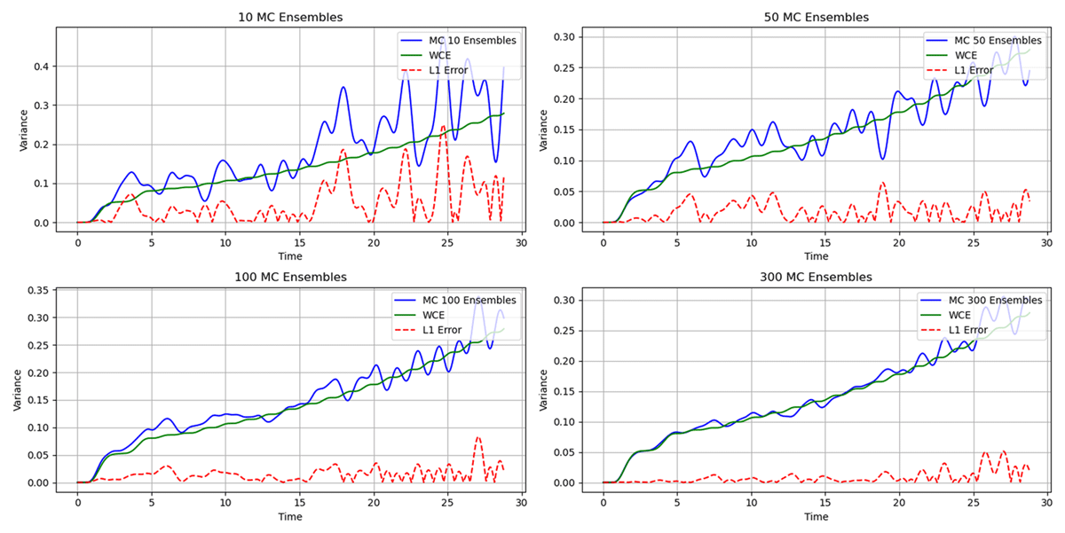
Figure 9
Comparison of WCE and MC variance results of with different number of ensembles at a fixed space point .
Figures 10, 11, and 12 depict the mean and variance the oceanic Kelvin wave , Rossby wave , and sea surface temperature using both WCE and MC methods. We only need the first (unforced) propagator solution for the WCE mean results, which takes 15 seconds. In contrast, the mean results for the MC simulations are obtained using 300 ensembles, requiring 4880 seconds. Although the error between these two methods is relatively small, the WCE method requires significantly less computation time to obtain the mean and variance solutions. As we make longer simulations, the error increases due to numerical inaccuracies. The variance of oceanic Kelvin and Rossby waves is confined in the first half of the ocean due to noise profile . The SST variance shifts towards the eastern part of the ocean, resulting in warmer water initiating El Niño events.
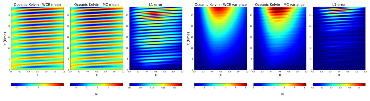
Figure 10
(a) Mean of oceanic Kelvin wave obtained from WCE (1st propagator), MC (300 ensembles), and the corresponding error. (b) Variance of oceanic Kelvin wave obtained from WCE (50 propagators), MC (300 ensembles).
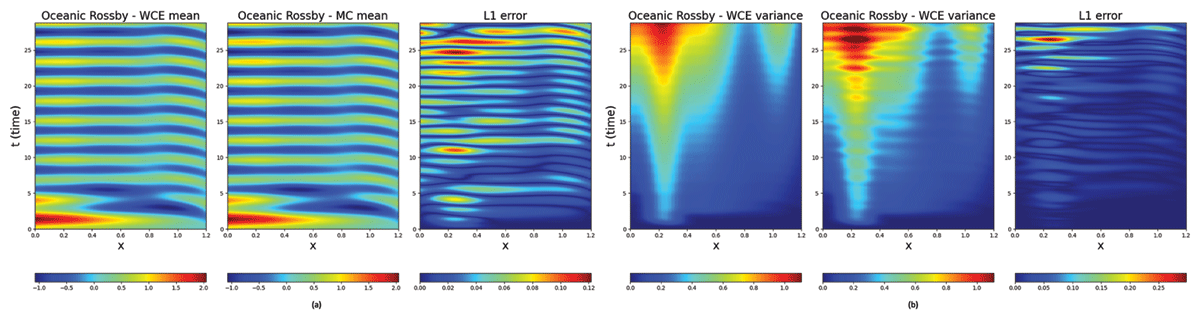
Figure 11
(a) Mean of oceanic Rossby wave obtained from WCE (1st propagator), MC (300 ensembles), and the corresponding error. (b) Variance of oceanic Rossby wave obtained from WCE (50 propagators), MC (300 ensembles).
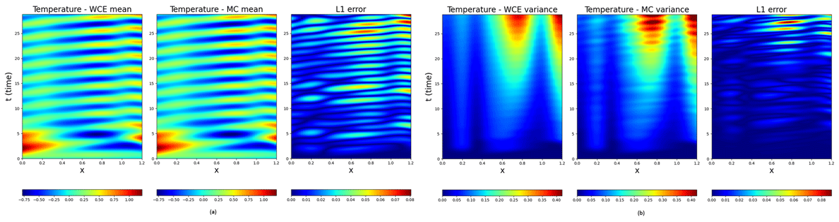
Figure 12
(a) Mean of sea surface temperature (SST) obtained from WCE (1st propagator), MC (300 ensembles), and the corresponding error. (b) Variance of sea surface temperature (SST) obtained from WCE (50 propagators), MC (300 ensembles).
5 Conclusion
In this paper, we delved into a stochastic climate model by the numerical simulations based on Wiener chaos expansion and Monte Carlo methods. The utilization of WCE provided a comprehensive study based on spectral approach while MC simulations enhanced our ability to analyze stochastic models through ensemble methods. Although WCE and MC based methods have been applied to many problems, this paper investigated a relatively uncommon application on the high dimensional coupled SPDE models.
Initially, we applied the WCE-based scheme on the simple ocean model formed by oceanic Kelvin and Rossby waves forced with white noise. The WCE approach with 10 propagators converged exact mean and variance values obtained from the method of characteristics with high accuracy. These results demonstrated that the WCE method would be an appropriate method for high dimensional and more complicated models. Subsequently, we utilized a linear stochastic ENSO model forced by the Ornstein-Uhlenbeck process to show the accuracy of the method. We compared the WCE results formed by 50 modes, which is assumed to be the benchmark for the solution, with 300 MC ensembles. We showed that the mean and variance results of the stochastic model based on MC method converges to the WCE results. Remarkably, the model simulation with WCE required less computational resources as opposed to MC ensembles. Along with the noise construction with specific model parameters, this work provides an alternative approach for simulations of stochastic climate models with accurate and less computational resources that can be considered as the first step of more complex and longer simulation.
Despite the fact that WCE provides several advantages both numerical and theoretical, it has its drawbacks. As WCE is applied to particularly high dimensional nonlinear problems, it becomes more computationally expensive due to the increasing number terms in the chaos expansions. The simulation of stochastic models involving non-Gaussian processes through WCE may not be the most efficient and effective approach. Depending on the type of problem, MC or other numerical methods can be more suitable.
Data Accessibility Statement
The datasets and code used to produce the results in this paper can be accessed at https://github.com/Y1Aydogdu/ENSO_WCE_MonteCarlo.git
Appendices
Appendix
Consider the boundary value problem related to the ENSO atmosphere equation
with boundary conditions . Here, is a given function of temperature, and r is a given constant, and we wish to find U that could be or . The general solution is
The boundary condition gives
so that
and hence
Let denote the solution to the ODE with the initial condition . Then
and so
Acknowledgements
The authors would like to thank Professor Peter Baxendale, Department of Mathematics, University of Southern California, for stimulating discussions, contributions, and suggestions on many topics of this paper.
Funding Information
The authors acknowledge partial support for this work from Natural Sciences and Engineering Research Council (NSERC) Discovery grant 50503-10802, TECSIS/Fields-CQAM Laboratory for Inference and Prediction, and NSERC-CRD grant 543433-19.
Competing Interests
The authors have no competing interests to declare.
Author Contributions
Each author has made the following contributions to the development of this manuscript: problem formulation—Yusuf Aydogdu, N. Sri Namachchivaya; simulation, analysis and interpretation of results—Yusuf Aydogdu; draft manuscript preparation—Yusuf Aydogdu; supervision and revision—N. Sri Namachchivaya.