
1. Introduction
Global warming, combined with changing climate change, stands as the main industrial revolution outcome, influencing energy demand, environmental sustainability, and economic stability (Lorente et al., 2023). Multiple deadly effects, including mortality rates, droughts, heat waves, glacier melting, and floods, result from global climate change (Rajak, 2021). Over the past few years, concerns have arisen that global climate change may lead to an increased risk of droughts. Droughtis defined as a deficit of water over certain years, and is a major consequence of global warming (Cook et al., 2020; Jehanzaib et al., 2020). Therefore, immediate attention is essential to accurately and precisely notify decision-makers, environmentalists, and hydrologists about drought characteristics (Batool et al., 2023). Studies have analyzed the effects of drought on the economy, agriculture, and water resources (Dost and Kasiviswanathan, 2023). The National Drought Mitigation Center (NDMC) defines drought through its official description as ‘a prolonged period of deficient rainfall leading to water scarcity’ (Yihdego, Vaheddoost and Al-Weshah, 2019). This is a multidimensional natural event that has serious effects on ecosystems, agriculture, water supplies, and entire populations. The manifestation of drought results from complex climate-related interplay that extends over broad geographical regions and longer periods than other climate-based natural hazards. Drought stands as one of the most damaging natural events economically (Mukherjee, Mishra and Trenberth, 2018; Ali et al., 2022). Drought events fall into four climatological classifications: hydrological, meteorological, agricultural, and socioeconomic (Wang et al., 2016). The management of drought impacts needs proper identification and evaluation of drought dynamics. Drought assessment and characterization require standardized toolkits as part of their process (Erhardt and Czado, 2018). Therefore, many researchers have developed numerous drought monitoring tools and indices (Ali et al., 2020; Ahmad et al., 2023). Svoboda and Fuchs (2016) discussed the most widely utilized drought indices in drought-prone regions for making informed decisions in early warnings. Furthermore, predicting drought attributes relies on probabilistic techniques combined with machine-learning approaches (Niaz et al., 2022). The use of a copula for drought assessment has been explored in earlier studies (Won et al., 2020; Tian et al., 2023).
More recently, Saha et al. (2023) developed a new drought monitoring strategy by using a deep learning algorithm in the West Bengal region of India. The development of a hybrid index based on an advanced machine-learning copula and a probability model is considered an accurate technique for monitoring drought characteristics (Jiang et al., 2023).
The accurate determination of drought characteristics remains one of the most difficult operations for local-level assessment. Previous studies have primarily focused on station-based drought assessments, which are often time-consuming and limited in scope due to resource constraints. Understanding climate characteristics by monitoring and evaluating droughts within specific areas is vital. Recently, Batool et al. (2023) introduced a novel index—the Standardized Composite Index for Climate Extremes (SCICE)—for regional drought assessment. Thus, aggregating individual distributions provides a more comprehensive representation of drought-related variables. The variability in extreme climate events, particularly the dynamic patterns of precipitation, remains one of the most challenging issues globally. To the best of our knowledge, no study has been conducted at the regional level in Turkey for an accurate and long-term assessment of drought behavior. The research aim is to correctly forecast upcoming drought profiles within the Konya Closed Basin (KCB), Turkey. Therefore, this study developed a new index, the Quality Boosted Regional Drought Index (QBRDI). The methodology of QBRDI is based on the research conducted by Ali et al. (2023). The implementation of QBRDI relies on ensemble data from nine stations to decrease the uncertainty that occurs with individual stations. Numerous statistical techniques, including non-parametric standardization, Mann–Kendall (MK) trend analysis and other approaches, have been used for drought assessment and consequence evaluation. In this application, nine meteorological stations in the Konya region of Turkey have been analyzed.
The structural outline of this paper is documented as follows: Section 2 presents the materials and methods, including the framework of study and different existing methods. Section 3 contains a summary of the obtained results alongside their subsequent evaluation. Section 4 provides the conclusion.
2. Materials and Methods
2.1. Study area and data collection
This study presents a thorough investigation of the KCB in Turkey. The central Anatolian semi-arid area in Turkey occupies an area of 53,850 km2 and holds special climatic conditions and ecological elements. The KCB region contains multiple drainage basins, while Tuz (Salt) Lake and Beysehir Lake achieve top status as Turkey’s largest freshwater lakes, serving as the region’s main water reservoirs. Drought monitoring tools are helpful for early warnings and mitigation policies. Several authors have suggested numerous drought indicators and monitoring tools to determine drought severity (Citakoglu & Coşkun, 2022; Soylu Pekpostalci et al., 2023). This study developed a new drought index (QBRDI) to assess the spatial-temporal distribution of drought in Turkey’s KCB region. The temporal dataset from nine meteorological stations in Turkey was collected and standardized before. Analyzed data originated from the General Directorate of Meteorology (MGM) of Turkey. Outliers were removed through a weighting scheme, where high weights were given to low values and low weights to high values, among other adjustments. Each station has 696 observations with a time frame of 57 years from 1965 to 2022. The spatial geographical distribution of these stations is provided in Figure 1 with geographic attributes—latitude, longitude, and altitude—while the observational view of these stations is shown in Figure 2. Table 1 presents details about the nine KCB stations in Turkey with geographic attributes—latitude, longitude, and altitude. This spread encompasses the expansive landscapes of the KCB, from vast plains to mountainous regions, in addition to its topographical shapes.
Table 1
Information about the nine meteorological stations in the Konya Closed Basin, Turkey.
| STATION NAME | LATITUDE (°N) | LONGITUDE (°E) | ALTITUDE (M) |
|---|---|---|---|
| Aksaray | 38.3705 | 33.9987 | 970 |
| Beysehir | 37.6777 | 31.7463 | 1141 |
| Cihanbeyli | 38.650578 | 32.92186 | 973 |
| Eregli | 37.5255 | 34.0485 | 1046 |
| Isparta | 37.7848 | 30.5679 | 997 |
| Karaman | 37.1932 | 33.2202 | 1018 |
| Konya | 37.9837 | 32.574 | 1031 |
| Nevsehir | 38.6163 | 34.7025 | 1260 |
| Nigde | 37.9587 | 34.6795 | 1211 |
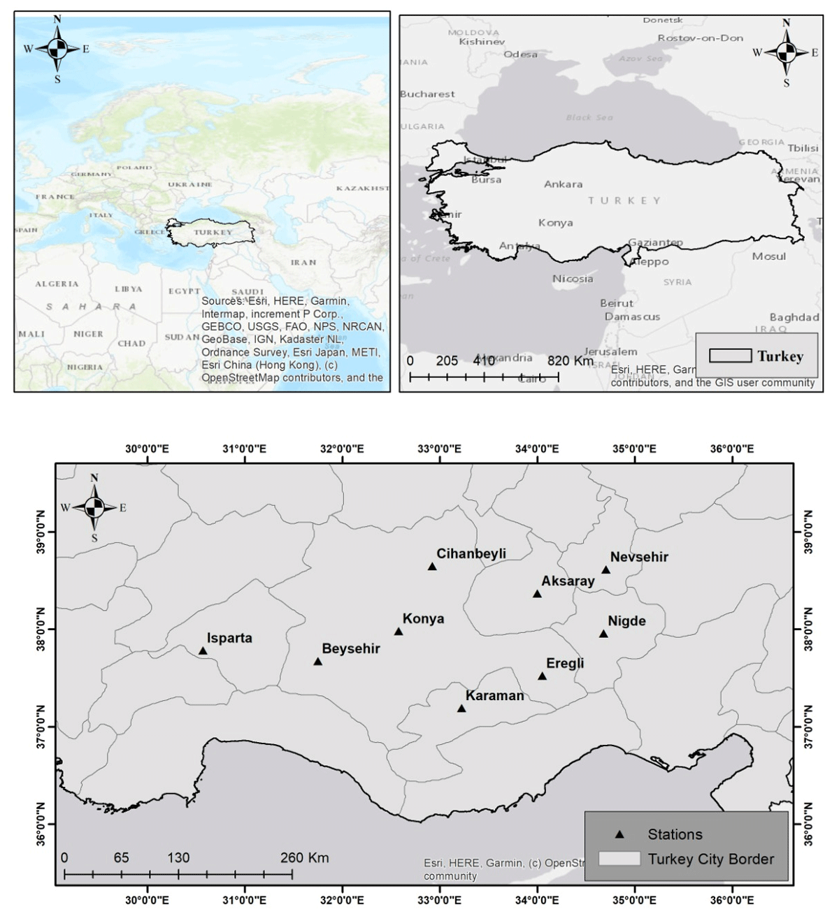
Figure 1
Map of the study site showing nine selected meteorological stations in the Konya Closed Basin located in Turkey.
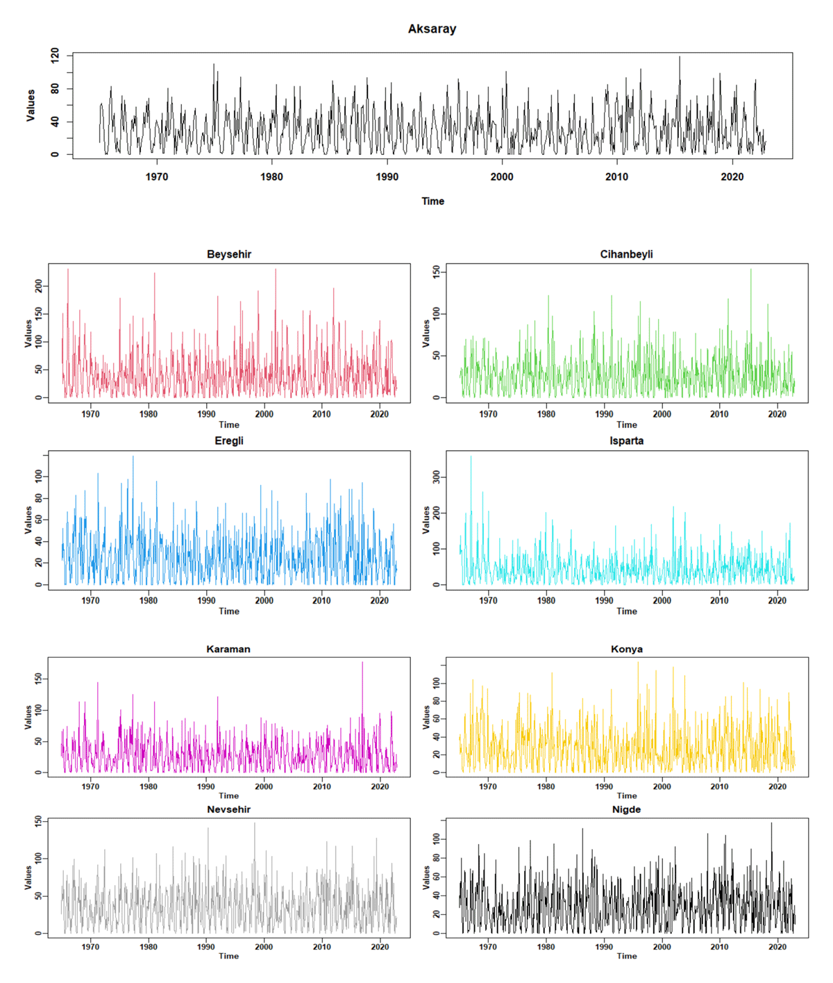
Figure 2
Temporal representation of selected nine meteorological stations in the Konya Closed Basin located in Turkey.
2.2. Probabilistic approach
Fitting an accurate and precise approach is essential for developing standardized drought indicators (Batool et al., 2024). Numerous methodologies have been employed in prior studies to achieve standardization objectives, with the most familiar ones being parametric and non-parametric techniques. In this study, two approaches, parametric and non-parametric, are utilized for standardization. Parametric approaches are the K-Component Gaussian Mixture Model (K-CGMM) (McLachlan & Peel, 2000) and univariate probability models. The univariate probability models are evaluated using the ‘fitDistr’ (Spiess, 2018) function from the Propagate package in R software. Univariate probability models are suitable for unimodal data. Previously, Abbas et al. (2022) used the ‘fitdistrplus’ and ‘Propagate’ package to fit distinct univariate distributions and selected the best one. Univariate probability models are not appropriate for fitting and computing cumulative distribution function (CDF) in the case of multimodal data. K-CGMM is an unsupervised technique utilized for modeling the multimodal data (Batool et al., 2025). K-CGMM is suitable for data that have numerous peaks. K-CGMM splits data into distinct components and fits a Gaussian distribution to each component of the data. It contains two parameters: weights and mean (or variance). For a concise and extensive overview of K-CGMM, see Batool et al. (2023). In some cases, the kth component shows zero variability, causing problems with K-CGMM. Then, determining CDF using a non-parametric technique leads to an accurate inference. The ultimate objective of each approach is to standardize QBRDI data by estimating the CDF from the underlying probability distributions. Hao and AghaKouchak (2014) employed non-parametric techniques to develop a multivariate standardized drought index (MSDI) for assessing drought behavior. Similarly, Ali et al. (2020) deployed the parametric approach in the context of drought assessment. After estimating the CDF using parametric or non-parametric techniques, standardization is performed based on the transformation outlined by Ali et al. (2017).
2.3. Trend analysis
2.3.1. Steady-state probability of Markov chain
Andrey Markov introduced the concept of Markov chains, a method involving steady-state probabilities (Markov, 1906). This study employed a first-order Markov chain, a discrete-time stochastic process that models how a random variable evolves at discrete points in time. In a first-order Markov chain, the probability of the future state depends solely on the present state, without considering earlier states. Therefore, this method is known as memoryless. The concept of compensating probabilities in Markov chains, developed by Keilson and Syski (1974), has received considerable attention in probability theory. It has broad applications across various real-world domains, including computer science, biology, and physics (Rajwar, Deep & Das, 2023). Markov chains have been employed to optimize the performance of different algorithms and to analyze population dynamics (Wang et al., 2020). A Markov chain examines the past transitory behavior of a process and contributes significantly to predicting uncertain phenomena. The mathematical framework of this method is built upon the transaction probability matrix (P), which plays a significant role in describing the behavior and transitions of Markov chains. This matrix captures the probabilities of transitioning from one state to another in the chain. In a Markov chain with k states, matrix P has an order of n × n, where each entry represents the probability of transitioning from state i to j in a one-time step (see Equation 1). The rows correspond to the current states, and the columns represent the possible subsequent states. Each value within the matrix ranges between 0 and 1, and the sum of each row or column should be equal to 1:
The elements in the matrix can be leveraged to quantify the stochastic state space’s transient probabilities. The long-term progression of system states is determined by the process’s limiting distribution or stationary probabilities, also known as steady-state probabilities.
2.3.2. MK test statistics
MK test, a widely used non-parametric method for detecting trends in temporal data, was originally developed by Mann (1945) and later refined by Kendall (1975) for more accurate trend assessment. This method compares both positive and negative trends in data collected over time. The MK test serves as an alternative to the parametric linear regression test, which fits a linear model to data and determines trend significance through model coefficients. The MK test has wide applications in economics, hydrology, and environmental sciences (Katipoğlu, 2023; Kheyruri et al., 2023). Researchers employ this technique to analyze temperature, precipitation, river flow, and stock market data trends (Reddy and Saravanan, 2023). The mathematical foundation of the test lies in the S statistic, which represents the signs of pairwise differences between each data point in the temporal series. The variance of this statistic is computed from the tied groups within the data, as illustrated in the equations below:
In the aforementioned calculations, xk and xl represent a time series that consists of n time points each. The parameter is used to denote the total count of distinct groups existing within the dataset, whereas specifically signifies the count of data points within the pth group.
2.3.3. Sen’s slope estimator
Sen’s slope is used to determine the magnitude of trends introduced by Sen. It was introduced for the first time by Sen (1968) also known as Sen’s estimator. This test has gained attention across various fields, including economics, ecological studies, and geophysics (Dost and Kasiviswanathan, 2023; Karanja et al., 2023). Furthermore, this test finds wide applications in analyzing groundwater levels and long-term economic indicators (Swain et al., 2022). In the environmental context, it monitors gradual changes in groundwater levels over time, providing insights into aquifer health (Fu et al., 2022). The calculation involves determining the median of slopes between data points. This is achieved by computing pairwise differences and dividing them by the time lag. The resulting median of these slopes provides a robust estimate of the trend, making it a suitable method for detecting trends even in the presence of outliers. The method uses a linear model to determine the slopes of residuals that remain constant throughout time. Mathematically,
where f(t) represents the function of the time series under the time period t, Q is the median of Sen’s slope estimator, and C represents the constant term.
The formula for Qi calculation is as follows:
where Q is the median of the slope at time l and m (m < l), and for M data points, the value of Q can be in two forms:
The positive value of the estimator implies a growing trend, while the negative value suggests a decrease in the trend, and the zero value indicates that no trend happened.
2.4. A framework of the study
The current study generates a drought monitoring index called the Quality Boosted Regional Drought Index (QBRDI) for the Konya region of Turkey, covering nine meteorological stations. The methodology of QBRDI is based on the previous study conducted by Ali et al. (2023). In QBRDI, we used an X-bar chart to identify out-of-control points (OCP). To aggregate regional data, weights are integrated based on the total number of OCP (TOCP). QBRDI is integrated into four different stages. The integration of each stage is presented below.
2.4.1. Stage 1. Implication of X-bar control chart to detect the OCP
The first stage of QBRDI examines the OCP based on an X-bar control chart. The upper control limit (UCL) and lower control limit (LCL) on the X-bar control chart are based on the averaged temporal data from meteorological stations in certain regions. The mathematical representation of this stage is as follows: let Mi be the temporal data of mean of selected stations. Let ¥ ∈ (LCL, UCL) be the lower and upper limits determined from Mi within X-bar chart. Let Ω ∈ (Total (OCP1), Total (OCP2), Total (OCP3), …, Total (OCPk)) signify the total values outside the control limits. Mathematically,
Here, n denotes the total number of points in the time series, and k represents the number of meteorological stations.
2.4.2. Stage 2. Determination of weights
This stage determines the weights for the mean of temporal data of selected meteorological stations. Weights are estimated based on the TOCP of each meteorological station. Let Ω ∈ (Total (OCP1), Total (OCP2), Total (OCP3), …, Total (OCPk)) signify the vector of total values outside the control limits within each station. It assigns lower weights to observations having a higher number of OCPs and vice versa. Mathematically,
where should be equal to 1, and k is the total number of meteorological stations.
2.4.3. Stage 3. Aggregation
In this stage, weights are assigned to the temporal data of precipitation for the aggregation. Let Di represent the time series data of precipitation at the ith meteorological station. The aggregated regional temporal precipitation data are obtained by weighting each station’s time series data according to their assigned weight. Mathematically,
where Ac represents the regional temporal data of precipitation within weight assignments, and Di is the time series precipitation data of the ith meteorological station.
2.4.4. Stage 4. Development of QBRDI standardization
After assigning weights to the datasets from all nine stations and constructing an ensemble model, the standardization of the QBRDI is assessed. The below mathematical expressions describe the structure of standardization (Ali et al., 2022):
where
when
and
where
when
where
where do= 2.515517, d1 = 0.802, d2 = 0.010328, e1 = 1.432788, e2 = 0.189269, and e3 = 0.001308 are the constants. The standardized data are classified into seven categories based on their values, ranging from extremely dry to extremely wet conditions. These classes are used to categorize drought severity based on standardized values. The classification provides a structured way to interpret drought conditions. The detailed information of seven standardized classes is as follows: extreme drought (ED): –2.00 and less, severe drought (SD): –1.50 to –1.99, moderate drought (MD): –1.00 to –1.49, near normal (NN): –0.99 to 0.99, moderate wet (MW): 1.00 to 1.49, severe wet (SW): 1.50 to 1.99, and extreme wet (EW): 2.00 and above.
2.5. Comparative methods and metrics
The weighting procedure in the development of QBRDI undergoes relative assessment within the utilization of the simple model average (SMA) procedure in this research. The cumulative index of the SMA follows this mathematical format:
where Si represents the ith precipitation observation at the meteorological station. The SMA method serves as a performance assessment approach, utilized by numerous researchers (Jose, Vincent & Dwarakish, 2022; Rhymee et al., 2022; Ombadi et al., 2021). This method is preferred due to its simplicity and ability to combine multiple results into a single index. Previous studies have discussed the limitations of SMA in comparison to more advanced, statistically rigorous methods, highlighting the need for approaches that account for the distribution and variance of the data. Therefore, we justify the use of SMA in this study as a baseline comparison for performance.
In this study, we have utilized the RMSE to determine the relative performance of weighted procedure utilized in QBRDI. Below is the presentation of mathematical expressions that define RMSE:
where Pi is the vector of the original dataset of precipitation, is the vector of predicted behavior, and k is the total number of selected stations.
The second performance metric is relative absolute error (RAE), which is also extensively employed in the literature. Mathematically,
where Pi is a vector of an actual data of precipitation and is the projection values. When comparing indexes, the lower RAE values indicate the superiority of one index over the other index.
3. Results and Discussion
3.1. Implication of weights and the validation of QBRDI
In this section, the results of weights under QBRDI and the validation of this index are defined. QBRDI aims to reduce bias and outliers and increase data reliability. Table 2 shows the monthly weights for all nine stations from January to December. QBRDI gives more weight to stations having lower number of OCP and less weight to stations having larger numbers of OCP and normalizes the dataset to investigate the drought characteristics. Figure 3 shows the temporal variation of all nine station weights QBRDI. It takes time on the x-axis (1965–2022) and weight values on the y-axis and shows the time difference between each model. The results presented in Table 3 demonstrate the superior performance of the deployed weighting procedure (Ali et al., 2023) compared to the SMA method. The RMSE values for the weighting procedure (Ali et al., 2023) are consistently lower across all three statistics—minimum, average, and maximum—indicating more accurate predictions. Specifically, the average RMSE under the weighting procedure (Ali et al., 2023) is 6.282, whereas SMA produces a much higher average RMSE of 15.158. Additionally, the maximum RMSE observed in QBRDI (8.618) is even lower than the minimum RMSE in SMA (7.333), highlighting the substantial improvement in predictive accuracy. Similarly, the RAE values show a significant reduction under the weighting procedure (Ali et al., 2023). The average RAE for the weighting procedure (Ali et al., 2023) is 0.085, while SMA results in an average RAE of 1.409, suggesting that the weighting procedure (Ali et al., 2023) provides more precise estimations and effectively captures variations in observed data. The superior performance of the weighting procedure (Ali et al., 2023) is attributed to its unequal weighting scheme, which assigns larger weights to stations having lower numbers of OCP and less weight to stations having larger numbers of OCP. Unlike SMA, which gives equal importance to all regions regardless of their reliability, QBRDI prioritizes more accurate regional analysis, leading to enhanced predictive accuracy. This dynamic weighting approach ensures that the ensemble is not influenced by poorly performing regions, reducing overall error. The significant reduction in RMSE and RAE validates the effectiveness of this method in improving drought index estimation. Thus, QBRDI emerges as a more robust and reliable alternative to SMA for ensemble modeling by incorporating a refined weighting strategy based on regional observation proximity.
Table 2
Monthly weights under QBRDI based on data from nine meteorological stations in the Konya Closed Basin, Turkey.
| STATIONS | JAN. | FEB. | MAR. | APR. | MAY | JUN. | JUL. | AUG. | SEP. | OCT. | NOV. | DEC. |
|---|---|---|---|---|---|---|---|---|---|---|---|---|
| Aksaray | 0.125 | 0.122 | 0.115 | 0.109 | 0.121 | 0.121 | 0.121 | 0.119 | 0.117 | 0.117 | 0.12 | 0.121 |
| Beysehir | 0.094 | 0.093 | 0.104 | 0.115 | 0.115 | 0.117 | 0.11 | 0.103 | 0.098 | 0.095 | 0.09 | 0.085 |
| Cihanbeyli | 0.114 | 0.119 | 0.115 | 0.103 | 0.114 | 0.115 | 0.113 | 0.113 | 0.113 | 0.114 | 0.117 | 0.12 |
| Eregli | 0.118 | 0.124 | 0.12 | 0.114 | 0.119 | 0.114 | 0.117 | 0.113 | 0.121 | 0.121 | 0.121 | 0.124 |
| Isparta | 0.069 | 0.085 | 0.099 | 0.094 | 0.086 | 0.103 | 0.088 | 0.087 | 0.096 | 0.096 | 0.087 | 0.076 |
| Karaman | 0.121 | 0.11 | 0.111 | 0.116 | 0.115 | 0.115 | 0.112 | 0.117 | 0.118 | 0.119 | 0.11 | 0.122 |
| Konya | 0.12 | 0.116 | 0.115 | 0.119 | 0.116 | 0.114 | 0.116 | 0.116 | 0.117 | 0.112 | 0.12 | 0.119 |
| Nevsehir | 0.116 | 0.111 | 0.102 | 0.111 | 0.097 | 0.09 | 0.106 | 0.113 | 0.106 | 0.107 | 0.116 | 0.112 |
| Nigde | 0.122 | 0.12 | 0.119 | 0.12 | 0.117 | 0.112 | 0.117 | 0.119 | 0.114 | 0.12 | 0.119 | 0.121 |
[i] Abbreviation: QBRDI, Quality Boosted Regional Drought Index.
Table 3
Validation of the deployed weighting procedure (Ali et al., 2023) using SMA.
| COMPARATIVE MEASURES | PROPOSED | SMA | ||||
|---|---|---|---|---|---|---|
| MINIMUM | AVERAGE | MAXIMUM | MINIMUM | AVERAGE | MAXIMUM | |
| RMSE | 2.618 | 6.282 | 8.618 | 7.333 | 15.158 | 27.752 |
| RAE | 0.043 | 0.085 | 2.266 | 0.679 | 1.409 | 2.712 |
[i] Abbreviations: RAE, relative absolute error; RMSE, root mean square error; SMA, simple model average.
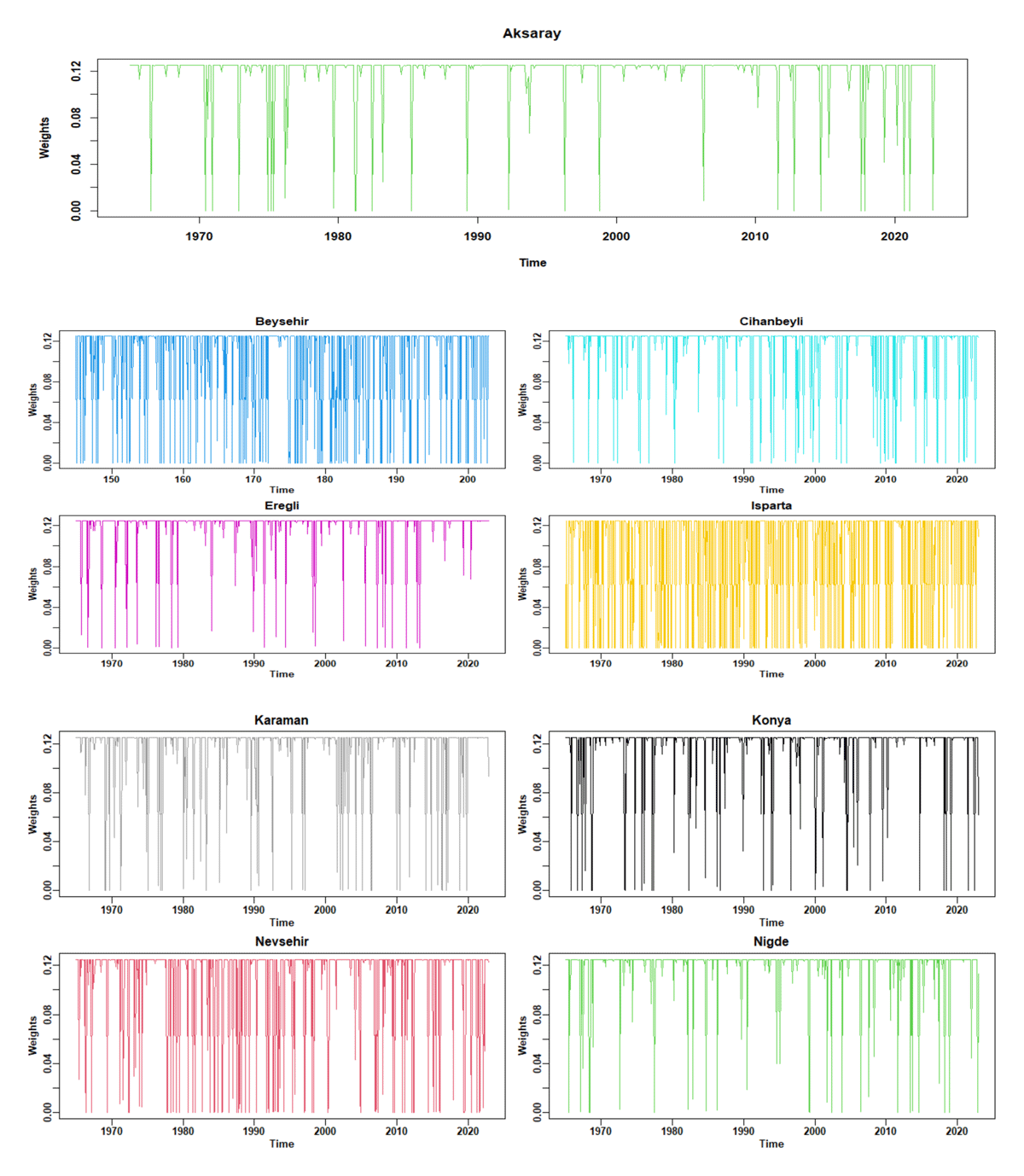
Figure 3
Temporal representation of weights of all nine meteorological stations in the Konya Closed Basin located in Turkey.
3.2. The implication of K-CGMM and non-parametric technique for standardization
In the present study, parametric and non-parametric approaches are used in the standardization process. The results presented in Table 4 highlight the superior performance of the K-CGMM compared to the univariate probability distributions in terms of the Bayesian Information Criterion (BIC) at various timescales. K-CGMM consistently outperforms univariate probability models, demonstrating its robustness in capturing the underlying behavior across most timescales. For instance, at timescale 1, the BIC for the univariate generalized normal distribution is –143.91, while K-CGMM achieves a significantly lower BIC of –645.13. Similarly, at scale 6, the univariate Johnson SB distribution has a BIC of –336.78, whereas K-CGMM drastically improves the fit with a BIC of –2608.2. These results confirm that K-CGMM provides a more efficient and accurate representation of the data distribution compared to traditional univariate models. However, at timescale 9, K-CGMM does not perform well, as evidenced by its higher BIC value (967.636) compared to the univariate Johnson SU model (–73.06). This suggests that the standard parametric approach for K-CGMM is not suitable at this timescale. To address this limitation, the CDF is determined non-parametrically, ensuring that the model remains flexible and accurately represents the distribution without imposing restrictive parametric assumptions. This adaptive approach allows K-CGMM to maintain its effectiveness across different timescales, even when standard parametric modeling does not provide an optimal fit. Overall, the results demonstrate that K-CGMM is a more effective modeling approach, as it consistently achieves lower BIC values, signifying better goodness-of-fit compared to univariate probability distributions. As depicted in Figure 4, the standardized data illustrate the temporal fluctuations during dry and wet conditions across seven distinct monthly timescales (1, 3, 6, 9, 12, 24, and 48). The y-axis represents standardized values, while the x-axis represents time. It signifies that data values from 0 to –2 show dryness and data values ranging from 0 to 2 show wetness.
Table 4
Evaluating appropriate distribution based on BIC under univariate distribution and K-CGMD at various timescales over single locations.
| SCENARIOS | QBRDI | ||
|---|---|---|---|
| TIMESCALES | UNIVARIATE PROBABILITY MODEL | K-CGMD | |
| Scale 1 | Generalized normal | –143.91 | –645.13 |
| Scale 3 | Johnson SU | –371.36 | –694.17 |
| Scale 6 | Johnson SB | –336.78 | –2608.2 |
| Scale 9 | Johnson SU | –73.06 | 967.636 |
| Scale 12 | Weibull | –470.35 | –1230.8 |
| Scale 24 | Generalized normal | –209.57 | –2134.6 |
| Scale 48 | 4P Beta | –172.36 | –235.02 |
[i] Abbreviations: BIC, Bayesian Information Criterion; QBRDI, Quality Boosted Regional Drought Index.
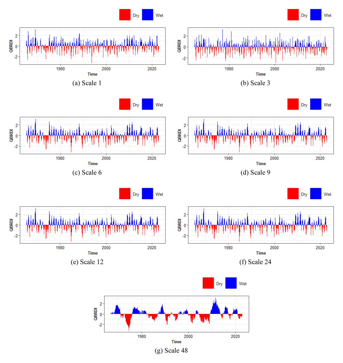
Figure 4
Temporal dry and wet fluctuation of QBRDI under seven different monthly timescales.
3.3. Assessment of long-term probabilities of drought and trend analysis
This section presents an overview of the long-term drought probability in Turkey’s KCB region, using a Markov chain steady-state probability model. The analysis is based on seven distinct classes representing varying drought and wet conditions. Table 5 presents the steady-state probability of seven classes at seven distinct timescales (1, 3, 6, 9, 12, 24, and 48). These values indicate the probability of various events occurring at each timescale. As we examine the probabilities from timescales 1 to 48, it becomes clear that the probabilities of ED and EW fluctuate slightly, with EW generally having lower probabilities.
Table 5
Steady-state probabilities for various drought classes under seven different timescales.
| TIMESCALES | ED | EW | MD | MW | NN | SD | SW |
|---|---|---|---|---|---|---|---|
| 1 | 0.023022 | 0.023022 | 0.090847 | 0.090647 | 0.683453 | 0.046604 | 0.044604 |
| 3 | 0.024089 | 0.023088 | 0.097352 | 0.092352 | 0.682540 | 0.043290 | 0.043290 |
| 6 | 0.023598 | 0.023102 | 0.093498 | 0.092408 | 0.680065 | 0.044014 | 0.043316 |
| 9 | 0.024100 | 0.023155 | 0.093031 | 0.091171 | 0.680164 | 0.044965 | 0.043415 |
| 12 | 0.023395 | 0.023392 | 0.095105 | 0.092105 | 0.681287 | 0.045860 | 0.043860 |
| 24 | 0.022324 | 0.022321 | 0.097262 | 0.092262 | 0.681548 | 0.047643 | 0.044643 |
| 48 | 0.023399 | 0.021836 | 0.093584 | 0.087345 | 0.689404 | 0.043673 | 0.040761 |
[i] Abbreviations: ED, extreme drought; EW, extreme wet; MD, moderate drought; MW, moderate wet; NN, near normal; SD, severe drought; SW, severe wet.
Meanwhile, MD and MW also exhibit fluctuations, with MD probabilities tending to be slightly higher than MW. NN shows a relatively stable probability of around 0.68 across all timescales. SD and SW exhibit similar patterns; both decrease as monthly timescales increase, and SW decreases continuously. Overall, the probabilities show that distinct timescales have varying impacts on these events, with some showing more stability than others. From these results, it can be concluded that KCB in Turkey may face drought problems in the future. To know the presence of a trend using two non-parametric techniques, Mann–Kendall and Sen’s slope. According to the MK test, a P value above the significance level (0.05) signifies an insignificant trend. Sen’s slope estimates this trend value; its sign indicates the direction of the trend. Table 6 provides trend analysis results for distinct timescales (i.e., 1, 3, 6, 9, 12, 24, and 48). For monthly timescales 1, 3, 6, and 9, the Kendall Z values and slopes are positive, indicating an increasing trend over time. However, these trends are generally relatively weak, as the slope values are small. For the 12- and 24-month timescales, both the Kendall Z values and slopes are negative, indicating a decreasing trend. Interestingly, at the 48-month timescale, the Kendall Z value and slope are positive, suggesting an increasing trend, but this time, the trend appears more prominent as the slope value is higher. These results suggest that there may be some fluctuations in the data, with both weak increasing and decreasing trends, but the most robust trend is observed with a significant positive slope at the 48-month timescale.
Table 6
Increasing and decreasing trend of drought under seven different monthly timescales.
| TIMESCALES | KENDAL Z | SLOPE | P VALUE | SIGNIFICANCE | DIRECTION |
|---|---|---|---|---|---|
| 1 | 0.42407789 | 0.000776753 | 0.671509 | P > 0.10 | Increasing |
| 3 | 0.4530965 | 0.000812574 | 0.6504793 | P > 0.10 | Increasing |
| 6 | 0.21919571 | 5.00E–04 | 0.8264976 | P > 0.10 | Increasing |
| 9 | 0.0059095 | 0.000126628 | 0.9952849 | P > 0.10 | Increasing |
| 12 | –0.20621246 | –0.0007875 | 0.836625 | P > 0.10 | Decreasing |
| 24 | –0.34809441 | –0.00112587 | 0.7277693 | P > 0.10 | Decreasing |
| 48 | 0.97762014 | 0.003484615 | 0.3282622 | P > 0.10 | Increasing |
4. Conclusion
Water is a vital element for human life and all other living creatures. Due to a lack of water, natural calamities such as droughts occur, which have devastating effects on various aspects of life. Therefore, there is an urgent need to develop new hybrid standardized methods to fully grasp the global effects of drought and water scarcity. In this regard, the present study used a newly developed regional drought index, QBRDI, to understand the drought consequences due to water shortage. In implementing QBRDI, this study utilized meteorological data spanning 57 years from nine stations to assess the drought characteristics within the KCB, located in Turkey. Furthermore, we employed the steady-state probabilities of the Markov chain to know the long-term evaluation of drought in the KCB region located in Turkey. The probability values obtained from this analysis were alarming, indicating the need to implement robust policies in this region to address future drought challenges. Two non-parametric techniques, namely the Mann–Kendall test and Sen’s slope estimator are employed to assess both the presence of a monotonic trend and the magnitude of that trend. Overall, the results show that while periods of SD have occurred, normal levels of drought are observed on average. Identification of wet and dry periods, along with trend analysis of meteorological data in the region, may assist in planning and managing regional water resources.
Data Accessibility Statement
The datasets used and/or analyzed in the present study are available from the corresponding author upon reasonable request.
Acknowledgements
A special thank you to Turkey’s General Directorate of Meteorology (MGM) for supplying the database utilized in this study.
Funding Information
Authors receive no funding for preparing this manuscript.
Competing Interests
The authors have no competing interests to declare.