
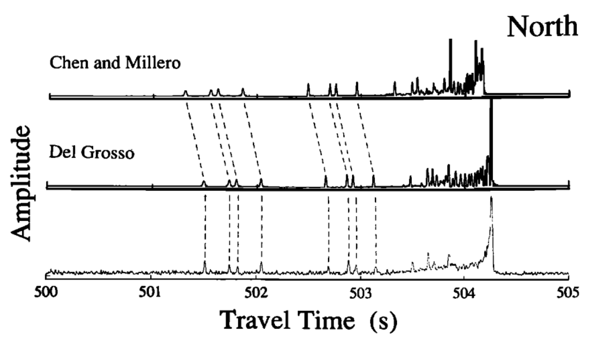
Figure 1
Acoustic arrival patterns measured over 750-km range in the central North Pacific in 1987 proved to be a precise test of the equations for the speed of sound in seawater (Dushaw et al. 1993a). The absolute travel time and dispersal pattern of the ray arrivals of the measured data are consistent with the Del Grosso sound speed equation. Such acoustic arrival patterns have proved to be stable and predictable throughout the world’s oceans. (From Dushaw et al. (1993a) by permission.)
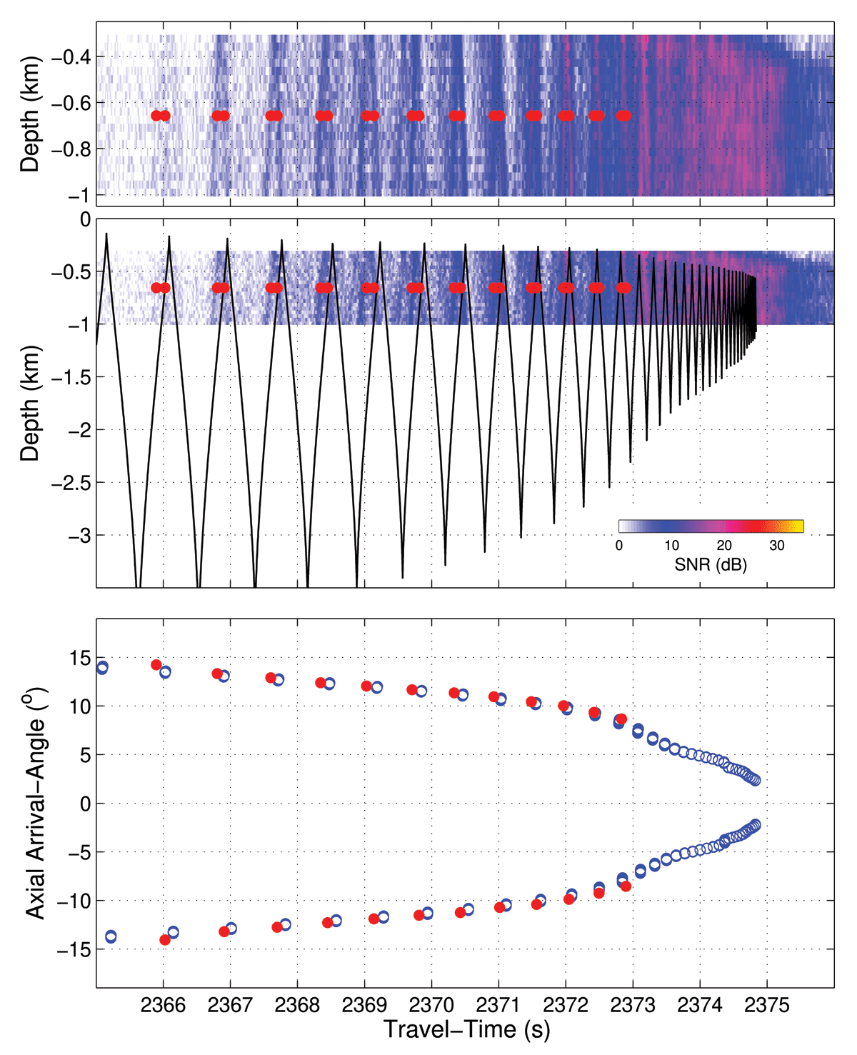
Figure 2
(top) The time front measured by a vertical line array near Hawaii from a transmission from Pioneer Seamount (3515-km range) on 15 May 1996. The red dots indicate the average travel times derived from the data. (middle) The measured time front compared to the time front calculated from the 2005 World Ocean Atlas (black lines). A travel time offset of +0.3 s has been applied to the predictions to achieve the alignment. (bottom) Comparison of measured (red dots) and predicted arrivals (blue circles) in vertical arrival angle versus travel time. (From (Dushaw et al. 2013) by permission.)
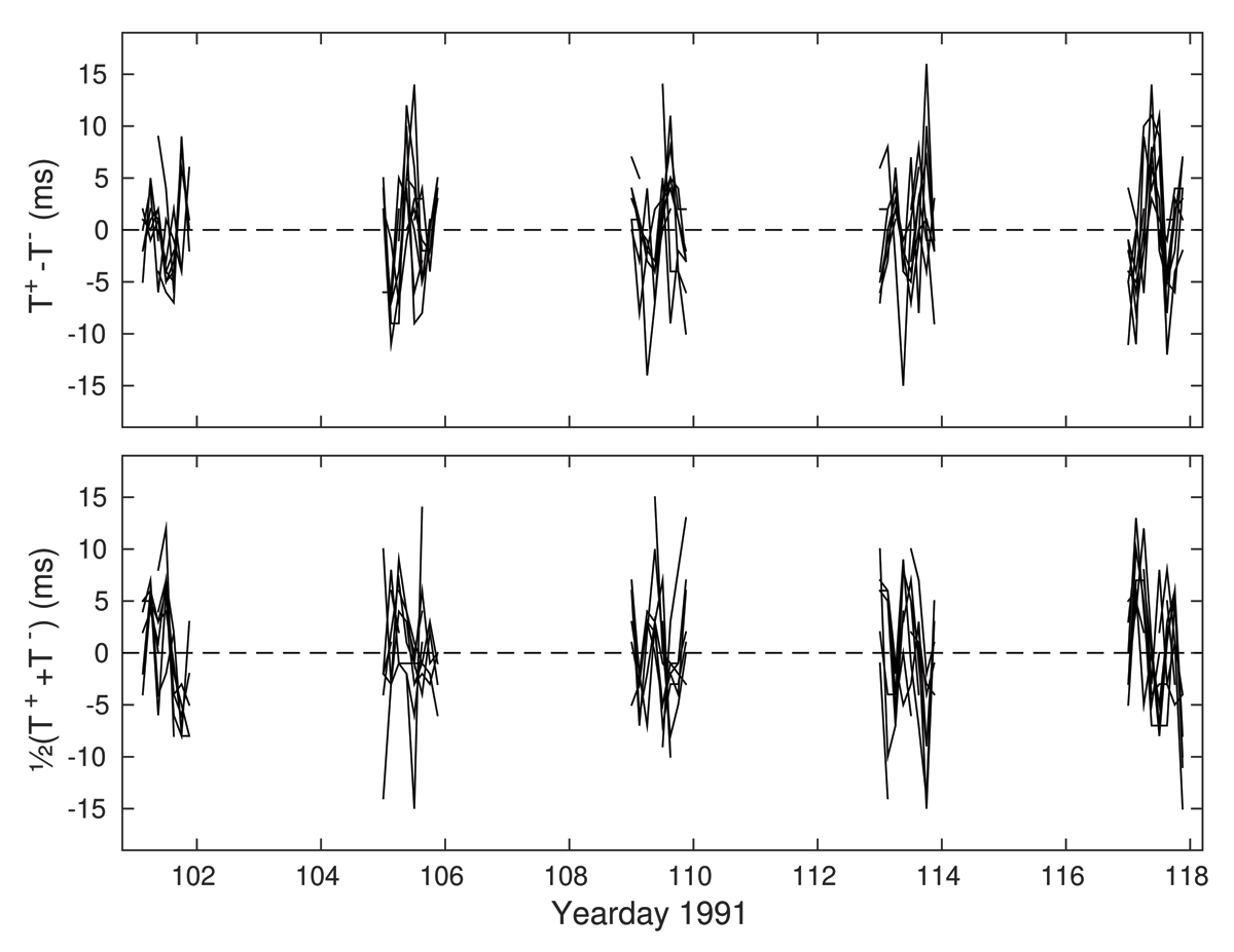
Figure 3
High-frequency (> 1 cpd) travel time variability measured during the 1991 Acoustic Mid-Ocean Dynamics Experiment (AMODE) on the 670-km acoustic path from mooring 1 to mooring 3. (Top) The difference of reciprocal travel times measures ocean current. The dominant signal of barotropic tidal currents is apparent. (Bottom) The sum of reciprocal travel times measures ocean temperature. The dominant signal of baroclinic tidal effects on temperature is apparent. The data of neither panel are filtered, other than the separation into high- and low-frequencies. The differential travel time data give accurate estimates of the tidal current harmonic constants. The sum travel time data, hardly different in character than the differential data, give accurate estimates of the tidal displacment harmonic constants (Dushaw 2006). Data such as these were first published in 1995 (Dushaw et al. 1995).
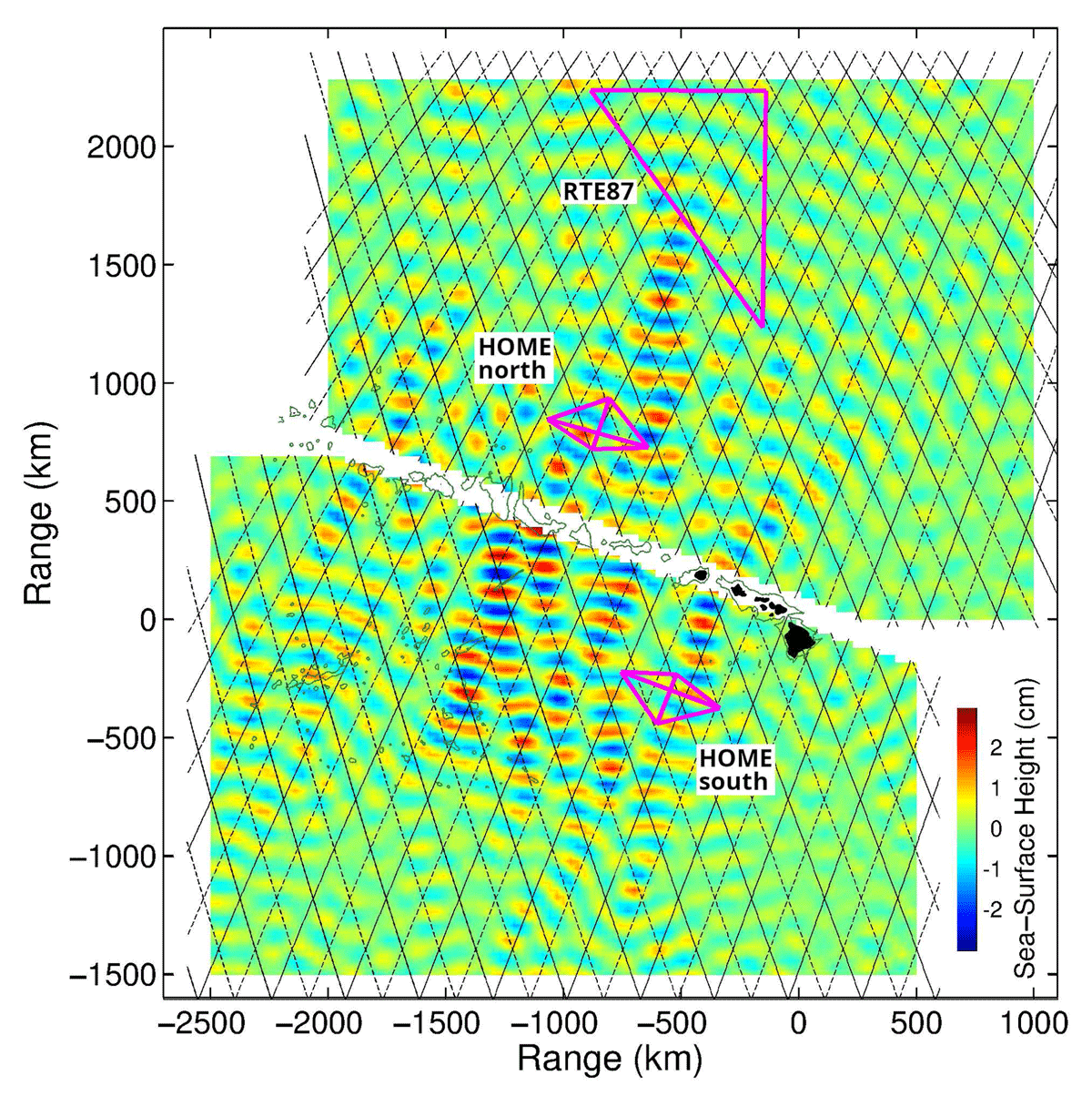
Figure 4
The locations of the RTE87 and HOME tomography experiments on either side of the Hawaiian Ridge. The colored field is the M2 internal tide sea-surface height derived from satellite altimetry data. The TOPEX/POSEIDON satellite tracks are indicated by the solid and dashed lines. Azimuthal Equal Area projection. (From Dushaw et al. (2011) by permission.) (See also electronic Supplements 1–3, D. Dushaw (2015a)).
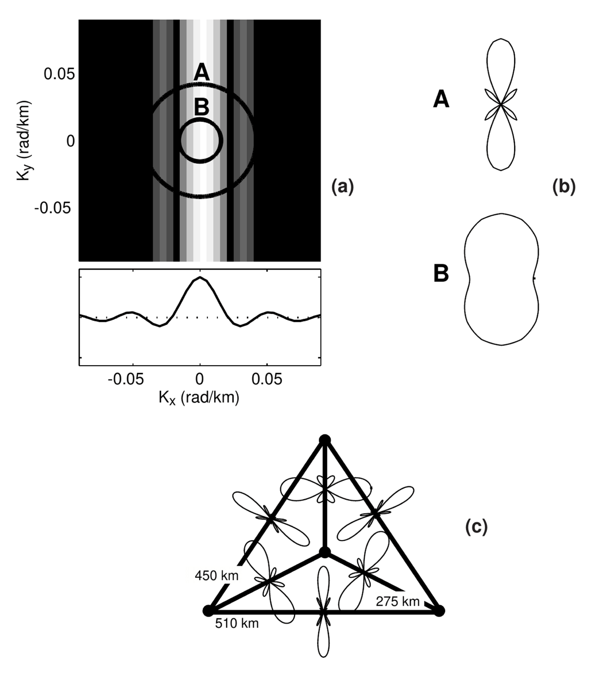
Figure 5
(a). A zonally-oriented acoustic path of 400-km length gives a sinc filter for zonal wavenumbers and no filter for meridional wavenumbers. (b). The projection of the two-dimensional filter onto semidiurnal wavenumbers A is the beam pattern (in polar coordinates), or the response of the line-integral antenna as a function of azimuthal angle, for semidiurnal radiation. The narrow beam pattern shows that the acoustic antenna has high directivity for semidiurnal wavenumbers. For the smaller diurnal wavenumbers B the acoustic antenna has less directivity. An acoustic tomography array (c) can be designed to provide for near-complete coverage of baroclinic-tide wavenumbers for waves traveling upward on the page. (From Dushaw (2003) © American Meteorological Society. Used with permission.)
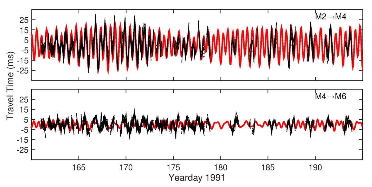
Figure 6
The tomography travel times recorded in the Atlantic in 1991 (black) can be independently predicted from a tidal analysis of altimetry data obtained a decade later (red) (Dushaw 2006; Dushaw et al. 2011; Dushaw 2015a). The two paths shown here have a mixed semidiurnal and diurnal signal (top) and a predominantly diurnal signal (bottom). The tomography data in this figure have been high-pass filtered only to distinguish between mesoscale and more rapid variability, i.e., these are the data, not just the tidal component of the data.
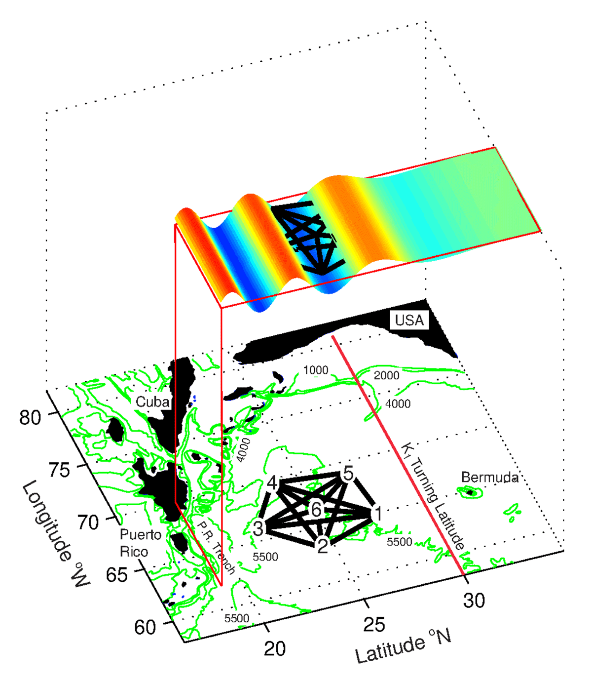
Figure 7
The AMODE tomography array observed relatively large, coherent K1 and O1 internal tides. Since the energy densities of the waves were far larger than expected from the weakness of the barotropic tides at those frequencies, such waves were interpreted as being in resonance, trapped between the Carribean island arc topography and their turning latitude at about 30°N (Dushaw and Worcester 1998; Dushaw 2006). (From Dushaw and Worcester (1998) by permission.)
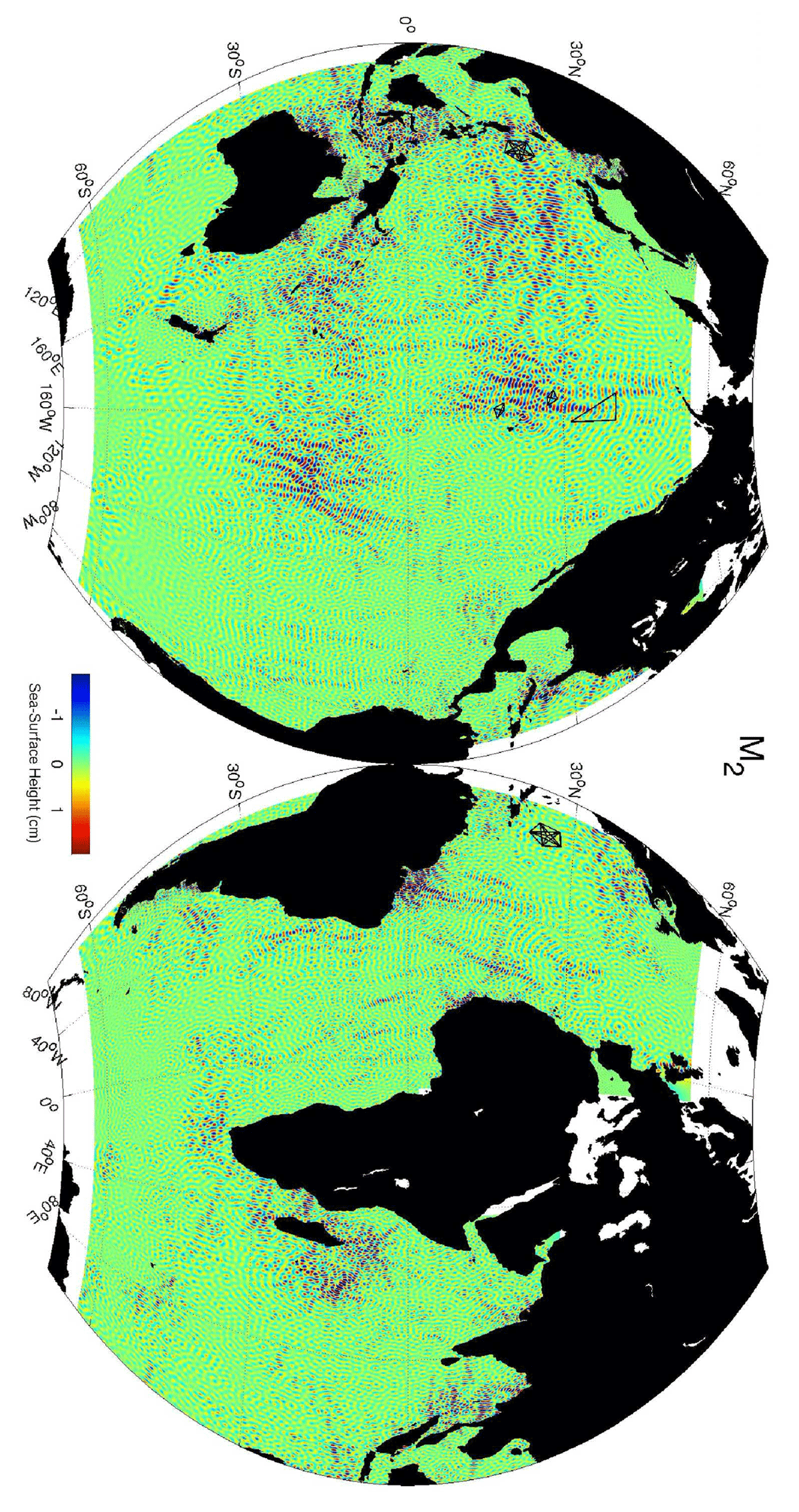
Figure 8
Sea-surface height of mode-1, M2 internal tide. From west to east tomography arrays are indicated in black lines: Philippine Sea, north and south arrays of HOME (Hawaii), RTE87 (central North Pacific), AMODE (Sargasso Sea). Hammer-Aitoff Projection. (From Dushaw (2015a).) (See also electronic Supplement 4.)
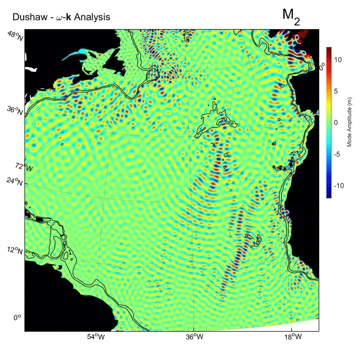
Figure 9
Mapping the internal-tide variability using the altimetry data allows some surprising wave features to be detected. By reconstructing the radiation using only generally southward wavenumbers, a long cylindrical wave train from the Azores almost to the coast of Brazil is revealed. The existence of such wave trains are a direct indication of the surprising spatial and temporal coherences of low-mode internal tides, since the complete wave field is a complicated interference pattern. Any incoherence would disrupt signals such as these. Units are internal-wave amplitude in meters, as computed from sea-surface height and solutions for internal-wave modes. (From Dushaw (2015a).) (See also electronic Supplement 5.)
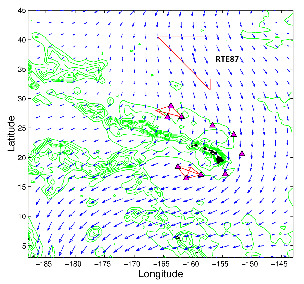
Figure 10
A schematic diagram of the farfield component of the HOME experiment. The arrows show the energy flux of the M2 barotropic tide; the barotropic tide prefers to go around the Hawaiian Ridge, rather than across it. By measuring barotropic tidal currents by tomography and tidal pressure by bottom tide gauges (magenta triangles) on either side of the Hawaiian Ridge, the aim was to determine the net tidal energy lost from the barotropic tide as it crossed over the Ridge. This energy goes into such processes as deep-ocean mixing or the radiation of internal tides away from Hawaii.
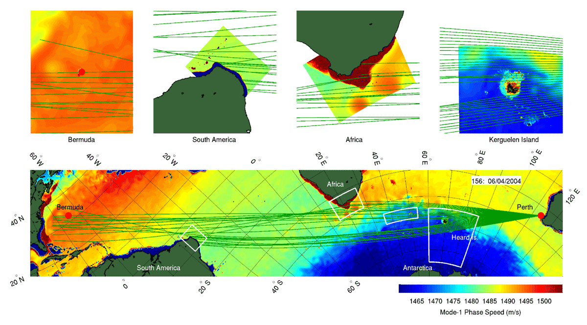
Figure 11
Computation of acoustic ray trajectories modeling the 1960 Perth to Bermuda acoustic propagation experiment. A fan of rays traced from Bermuda gave trajectories determined by oceanic refraction and scattering from topographic features. The colors indicate acoustic mode-1 phase speed for 15-Hz acoustic frequency derived from an ECCO ocean state estimate. Most rays either terminated at continental boundaries or passed south of Bermuda. Most often rays that arrived at Bermuda had scattered from topographic features in some way. The upper panels show the topographic interaction in detail: Kerguelen and the Crozet Islands were near perfect scatterers, the African continental shelf was a near perfect refractor, while the Brazilian continental shelf was a near perfect reflector. (From Dushaw (2014) by permission.) (See also electronic Supplement 6, the annimation of this figure mentioned by Munk (2011).)
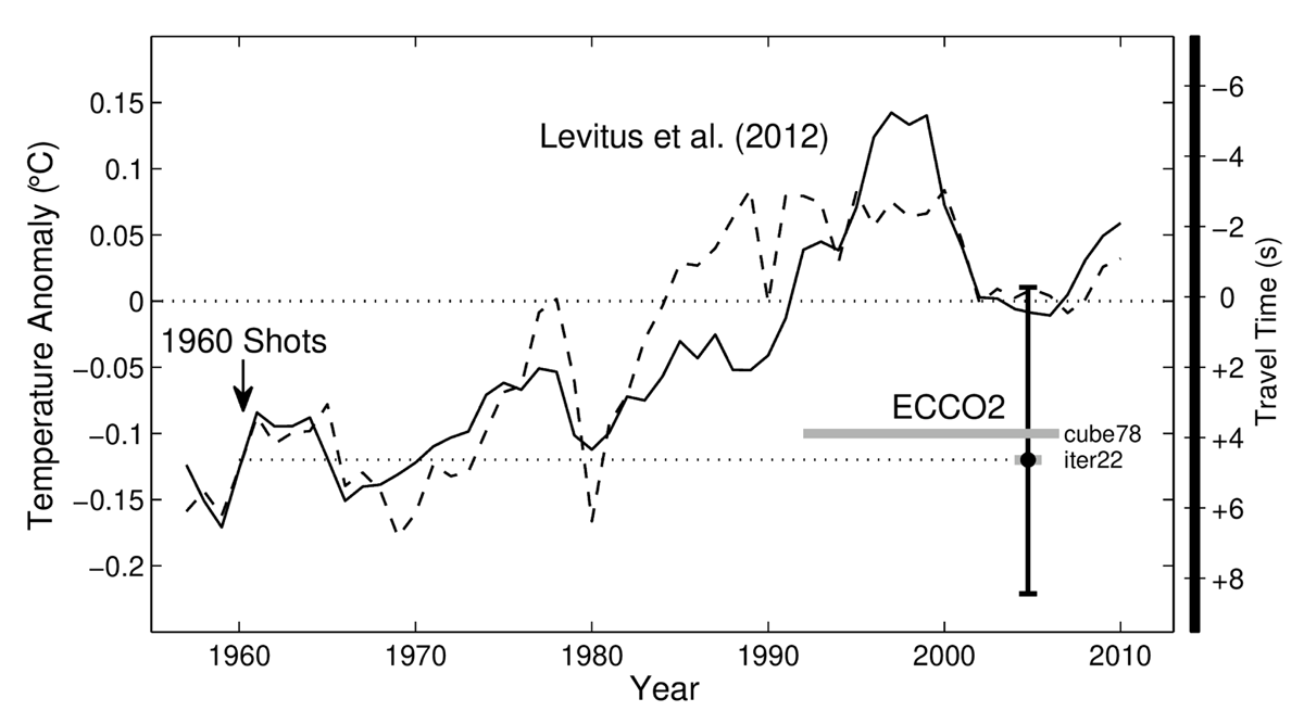
Figure 12
Time series of temperature anomaly over five decades computed by averaging the Levitus et al. (2021) estimates near the sound channel axis over antipodal acoustic paths (great circle/dashed, geodesic/solid). In these time series, the expected travel time decrease from 1960 to 2004 is only about 5 s, but the uncertainties are large. The intervals of the 15-year cube78 and 16-month iter22 ECCO2 solutions are indicated by the heavy gray lines, relative to the temperature anomaly value for 1960. Travel times computed from the state estimates were little changed from the 1960 measurements, but the uncertainties associated with the comparisons (–4.9/+3.8 s) are comparable to the warming signal expected from Levitus et al. (2012). (From Dushaw (2014) by permission.)
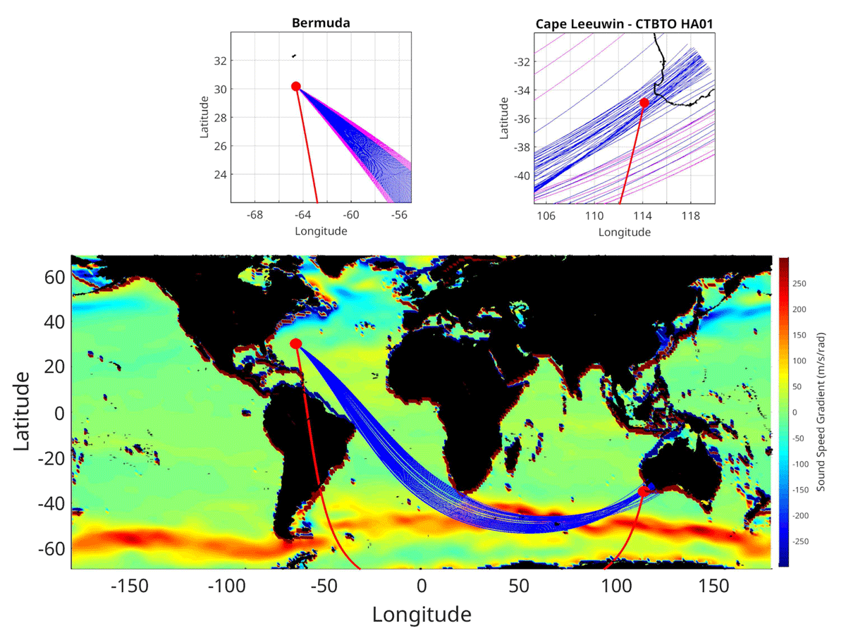
Figure 13
Refracted acoustic paths from a hypothetical 30-Hz acoustic source located about 200 km south of Bermuda arrive at the CTBTO hydroacoustic array HA01 off Cape Leeuwin, Australia. In the top panels, paths that intersect the South American or African continents are noted in magenta. The refraction is modeled using the first acoustic mode phase speed computed from the World Ocean Atlas; the colors indicate the meridional gradient of phase speed. The geodesic path is noted in red; the source and receiver are separated by slightly further than antipodal.
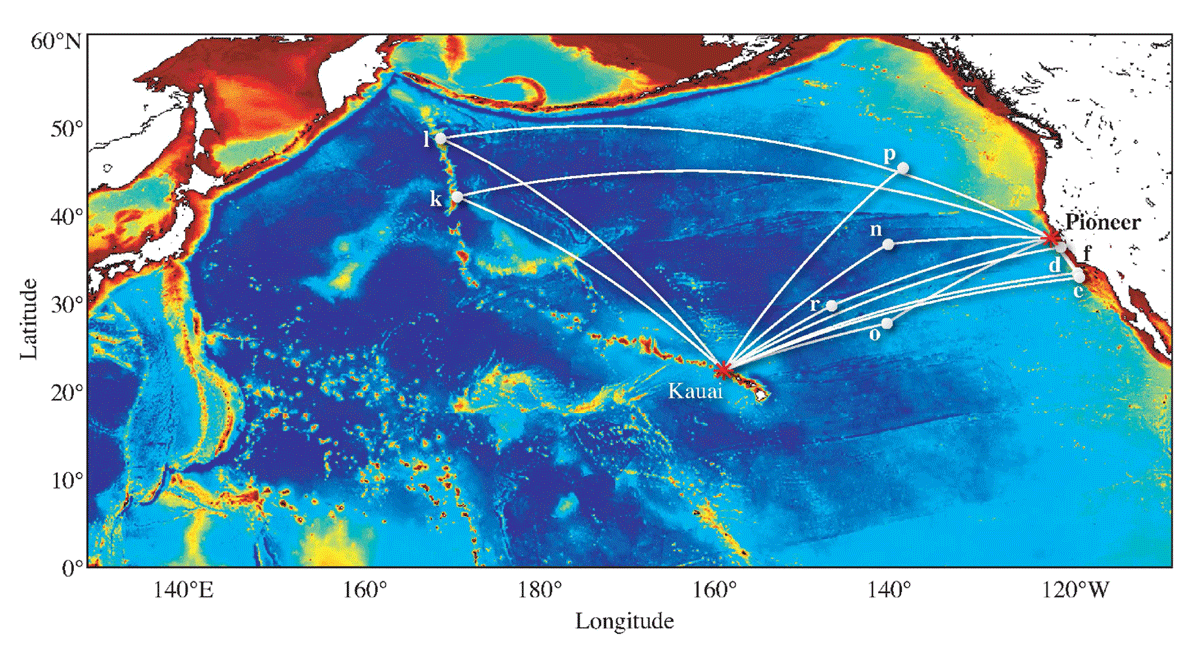
Figure 14
Acoustic paths from the 1996–2006 Acoustic Thermometry of Ocean Climate (ATOC) experiment. The acoustic source located on Pioneer Seamount transmitted for about a year, while the source located north of Kauai transmitted over a decade. Nominal receiver locations are denoted by letters. Data obtained from the Kauai to “k” path is shown in the next figure. (From Dushaw et al. (2009) by permission.)
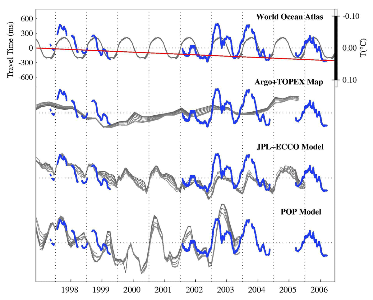
Figure 15
Comparison of measured travel times for transmissions from the source near Kauai to receiver k (blue) with travel times calculated using sound speed fields derived from: WOA05, estimates of upper-ocean temperature profiles produced by an OA procedure that combines satellite altimetric height with in situ temperature profiles, the JPL-ECCO solutions, and the POP model (gray). The time means have been removed from all of the time series. Approximate estimates of temperature perturbations averaged along the ray path inferred from the travel times are shown on the right-hand axis. The nominal travel time trend corresponding to a warming of 5 m°C/yr on the sound channel axis, as suggested by Munk and Forbes (1989), is shown (red). (From Dushaw et al. (2009) by permission.)
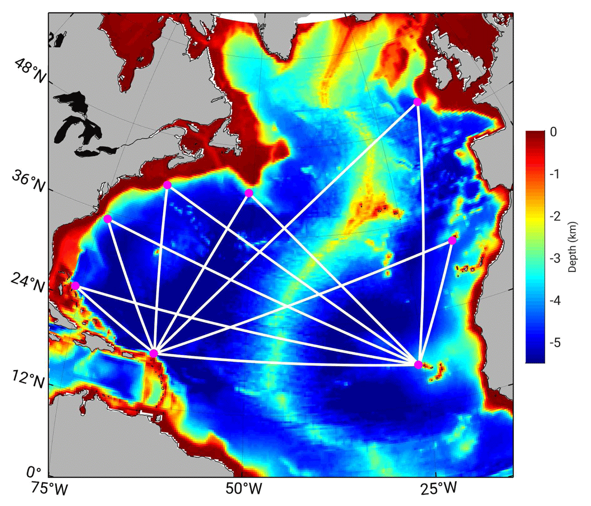
Figure 16
A hypothetical acoustic array for observing the North Atlantic Basin. This notional array consists of two acoustic sources and seven receivers. All instruments are located near a shelf break. One acoustic source is located near Antigua and Barbuda, another near the Cape Verde Islands. The acoustic paths are selected to avoid topographic interaction. An observing system consisting of such an array and Argo floats would significantly reduce the uncertainties of ocean state estimates at the largest scales compared to using a system of Argo floats alone. (From Dushaw (2019) © American Meteorological Society. Used with permission.)
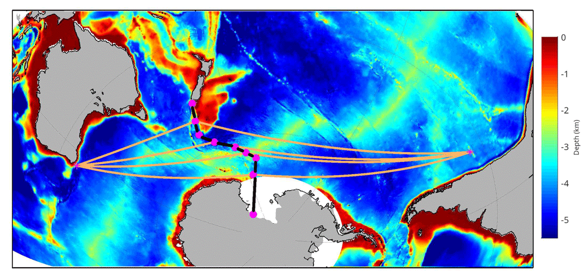
Figure 17
A hypothetical acoustic observing system for the Southern Ocean. This notional array would rely on hydrophones deployed on a planned communications cable between southern New Zealand and McMurdo Station, Antarctica. The acoustic paths shown, from 5000 to 7500 km in length, are from notional sources off Cape Leeuwin, Australia and Juan Fernandez, Chile.