
Table 1
Types of Localisations. Bottom 3 rows show localisation application novel to this paper. Cost functions are given in terms of the parameter θ which represents the parameters of the distribution.
| LOCALISATION | COST FUNCTION | FORM | BASED ON |
| Gaussian | NA | Damps sample covariance towards 0. | Tuned width parameter γ. The distance between 2 points dij. |
| Optimal for a single covariance (OSTC) | Damps sample sparse gain towards 0. | Signal: (mean) sparse gain. Noise: mean variance in sample sparse gain. | |
| Optimal for a variable covariance (OVTC) | Damps sample sparse gain towards 0. | Signal: mean and variance in sparse gain. Noise: mean variance in sample sparse gain. | |
| hybrid Optimal for a variable covariance (HOVTC) | Damps sample sparse gain towards mean sparse gain. | Signal: variance in sparse gain. Noise: mean variance in sample sparse gain. | |
| hybrid tuned double Gaussian (HTDG) | NA | Damps sample covariance towards mean covariance. | Tuned width parameters γ1 and γ2. The distance between 2 points dij. |
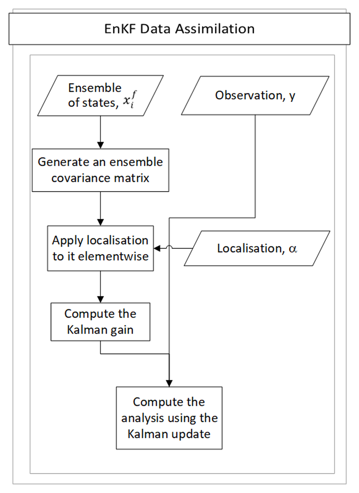
Figure 1
Schematic of a single DA process using the EnKF.
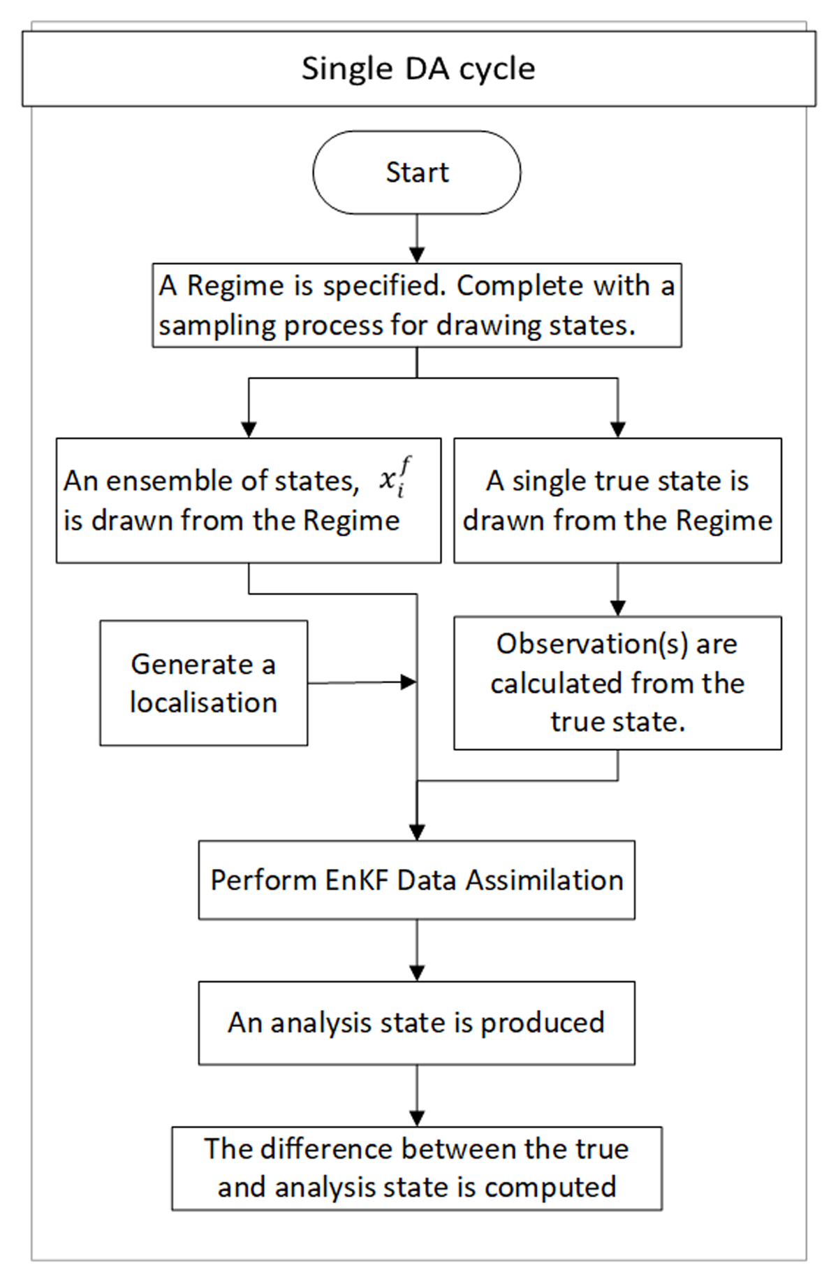
Figure 2
Schematic showing the ensemble and observation generation, assimilation and error production for a single DA cycle.
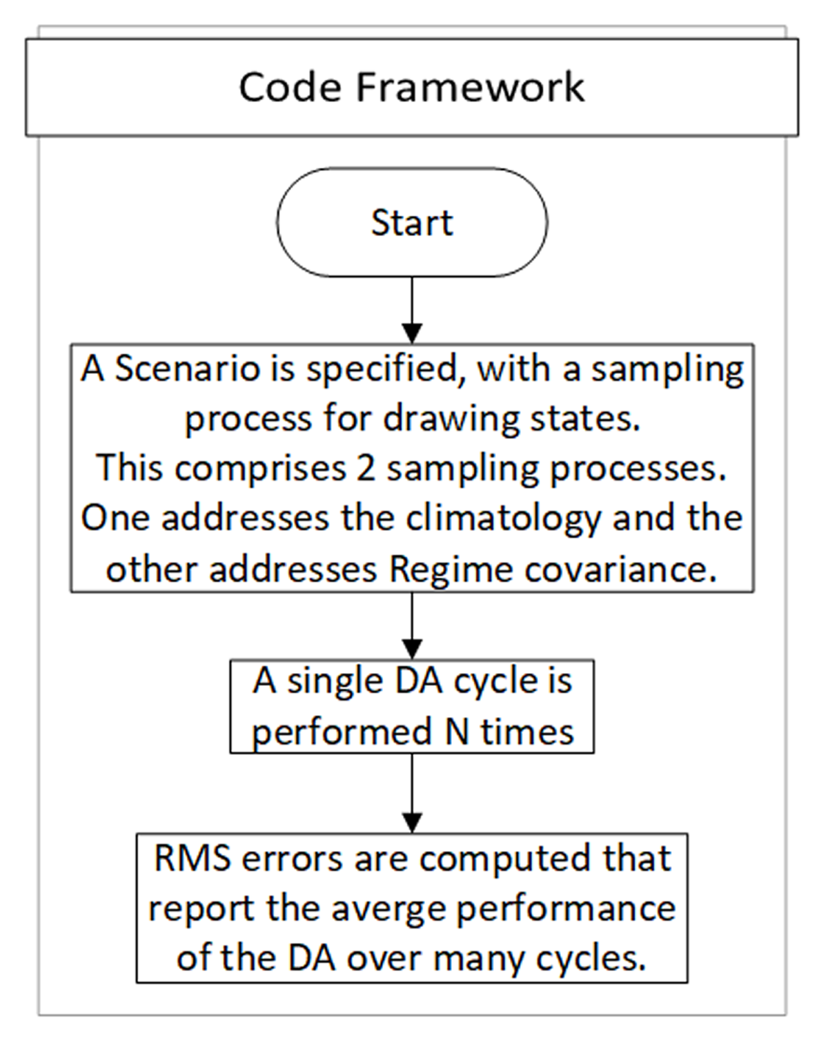
Figure 3
The flow diagram of the experiments performed and reported in this paper.
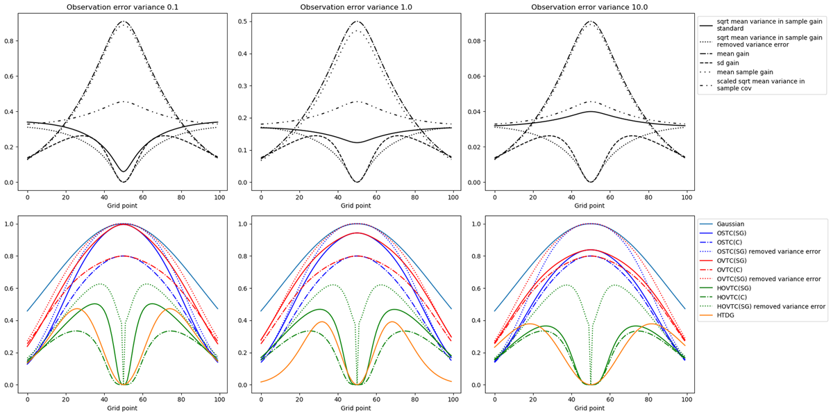
Figure 4
Plot showing the shape of each localisation and the statistics used to compute the localisation for Scenario 1. The form of the localisations is shown for observation variance 0.1, 1.0 and 10.0. The shown tuned widths are tuned from assimilating a single observation.
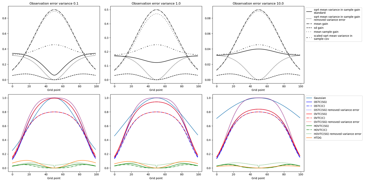
Figure 5
Plot showing the shape of each localisation and the statistics used to compute the localisation for Scenario 2. The form of the localisations is shown for observation variance 0.1,1.0 and 10.0. The shown tuned widths are tuned from assimilating a single observation.
Table 2
RMS error results for Scenario 1.
| SCENARIO 1 OBSERVATION ERROR VARIANCE 0.1 | ||||||||||||
|---|---|---|---|---|---|---|---|---|---|---|---|---|
| OSTC | OVTC | HOVTC | ||||||||||
| GAUSSIAN | (SG;G) | (C;C) | (SG;C) | (SG;G) | (C;C) | (SG;C) | (SG;G) | (C;C) | (SG;C) | HTDG | BACKGROUND ERROR | |
| Single ob | 0.8633 | 0.8656 | 0.8647 | 0.8656 | 0.8634 | 0.8631 | 0.8633 | 0.8522 | 0.8557 | 0.8576 | 0.8558 | 1.0466 |
| Spacing 33 | 0.5368 | 0.5525 | 0.5376 | 0.5366 | 0.5523 | 0.5402 | 0.5375 | 0.5804 | 2.4186 | 14.7818 | 0.5233 | 1.0462 |
| Spacing 9 | 0.2440 | 0.2852 | 0.2468 | 0.4289 | 0.2855 | 0.2613 | 0.2449 | 1.8869 | 212.2495 | 38.626 | 0.2573 | 1.0461 |
| SCENARIO 1 OBSERVATION ERROR VARIANCE 1.0 | ||||||||||||
| OSTC | OVTC | HOVTC | ||||||||||
| GAUSSIAN | (SG;G) | (C;C) | (SG;C) | (SG;G) | (C;C) | (SG;C) | (SG;G) | (C;C) | (SG;C) | HTDG | BACKGROUND ERROR | |
| Single ob | 0.9480 | 0.9502 | 0.9523 | 0.9498 | 0.9490 | 0.9506 | 0.9487 | 0.9398 | 0.9410 | 0.9411 | 0.9417 | 1.0466 |
| Spacing 33 | 0.7848 | 0.7947 | 0.7911 | 0.7860 | 0.7927 | 0.7901 | 0.7854 | 0.7698 | 0.7668 | 0.7682 | 0.7669 | 1.0462 |
| Spacing 9 | 0.5633 | 0.5886 | 0.5701 | 0.5641 | 0.5870 | 0.5709 | 0.5642 | 1.1460 | 0.5931 | 4.6481 | 0.5493 | 1.0461 |
| SCENARIO 1 OBSERVATION ERROR VARIANCE 10.0 | ||||||||||||
| OSTC | OVTC | HOVTC | ||||||||||
| GAUSSIAN | (SG;G) | (C;C) | (SG;C) | (SG;G) | (C;C) | (SG;C) | (SG;G) | (C;C) | (SG;C) | HTDG | BACKGROUND ERROR | |
| Single ob | 1.0277 | 1.0283 | 1.0285 | 1.0283 | 1.0280 | 1.0282 | 1.0280 | 1.0252 | 1.0253 | 1.0253 | 1.0253 | 1.0466 |
| Spacing 33 | 0.9977 | 0.9992 | 0.9993 | 0.9988 | 0.9985 | 0.9987 | 0.9982 | 0.9903 | 0.9906 | 0.9906 | 0.9911 | 1.0462 |
| Spacing 9 | 0.9152 | 0.9220 | 0.9197 | 0.9184 | 0.9203 | 0.9184 | 0.9173 | 0.9031 | 0.8989 | 0.8989 | 0.8992 | 1.0461 |
Table 3
RMS error results for Scenario 2.
| SCENARIO 2 OBSERVATION ERROR VARIANCE 0.1 | ||||||||||||
|---|---|---|---|---|---|---|---|---|---|---|---|---|
| OSTC | OVTC | HOVTC | ||||||||||
| GAUSSIAN | (SG;G) | (C;C) | (SG;C) | (SG;G) | (C;C) | (SG;C) | (SG;G) | (C;C) | (SG;C) | HTDG | BACKGROUND ERROR | |
| Single ob | 0.8311 | 0.8296 | 0.8295 | 0.8295 | 0.8295 | 0.8295 | 0.8294 | 0.8068 | 0.8068 | 0.8068 | 0.8070 | 1.0469 |
| Spacing 33 | 0.3701 | 0.3858 | 0.3763 | 0.3745 | 0.3856 | 0.3758 | 0.3739 | 0.5856 | 0.3495 | 0.3460 | 0.3459 | 1.0464 |
| Spacing 9 | 0.1995 | 0.2175 | 152.6382 | 136.7548 | 0.2174 | 16.2293 | 109.381 | 3.4972 | 0.1947 | 0.1947 | 0.1940 | 1.0463 |
| SCENARIO 2 OBSERVATION ERROR VARIANCE 1.0 | ||||||||||||
| OSTC | OVTC | HOVTC | ||||||||||
| GAUSSIAN | (SG;G) | (C;C) | (SG;C) | (SG;G) | (C;C) | (SG;C) | (SG;G) | (C;C) | (SG;C) | HTDG | BACKGROUND ERROR | |
| Single ob | 0.9324 | 0.9329 | 0.9350 | 0.9326 | 0.9329 | 0.2349 | 0.9326 | 0.9161 | 0.9161 | 0.9161 | 0.9161 | 1.0469 |
| Spacing 33 | 0.7279 | 0.7370 | 0.7352 | 0.7289 | 0.7370 | 0.7352 | 0.7288 | 0.7215 | 0.6971 | 0.6971 | 0.6971 | 1.0464 |
| Spacing 9 | 0.5089 | 0.5280 | 0.5173 | 0.5119 | 0.5280 | 0.5170 | 0.5113 | 1.8282 | 0.4846 | 0.4846 | 0.4847 | 1.0463 |
| SCENARIO 2 OBSERVATION ERROR VARIANCE 10.0 | ||||||||||||
| OSTC | OVTC | HOVTC | ||||||||||
| GAUSSIAN | (SG;G) | (C;C) | (SG;C) | (SG;G) | (C;C) | (SG;C) | (SG;G) | (C;C) | (SG;C) | HTDG | BACKGROUND ERROR | |
| Single ob | 1.0253 | 1.0252 | 0.0254 | 1.0252 | 1.0252 | 1.0254 | 1.0252 | 1.0207 | 1.0207 | 1.0207 | 1.0207 | 1.0469 |
| Spacing 33 | 0.9897 | 0.9904 | 0.9907 | 0.9902 | 0.9904 | 0.9907 | 0.9901 | 0.9780 | 0.9782 | 0.9782 | 0.9782 | 1.0464 |
| Spacing 9 | 0.8941 | 0.8998 | 0.8982 | 0.8969 | 0.8997 | 0.8982 | 0.8968 | 0.8882 | 0.8706 | 0.8706 | 0.8707 | 1.0463 |
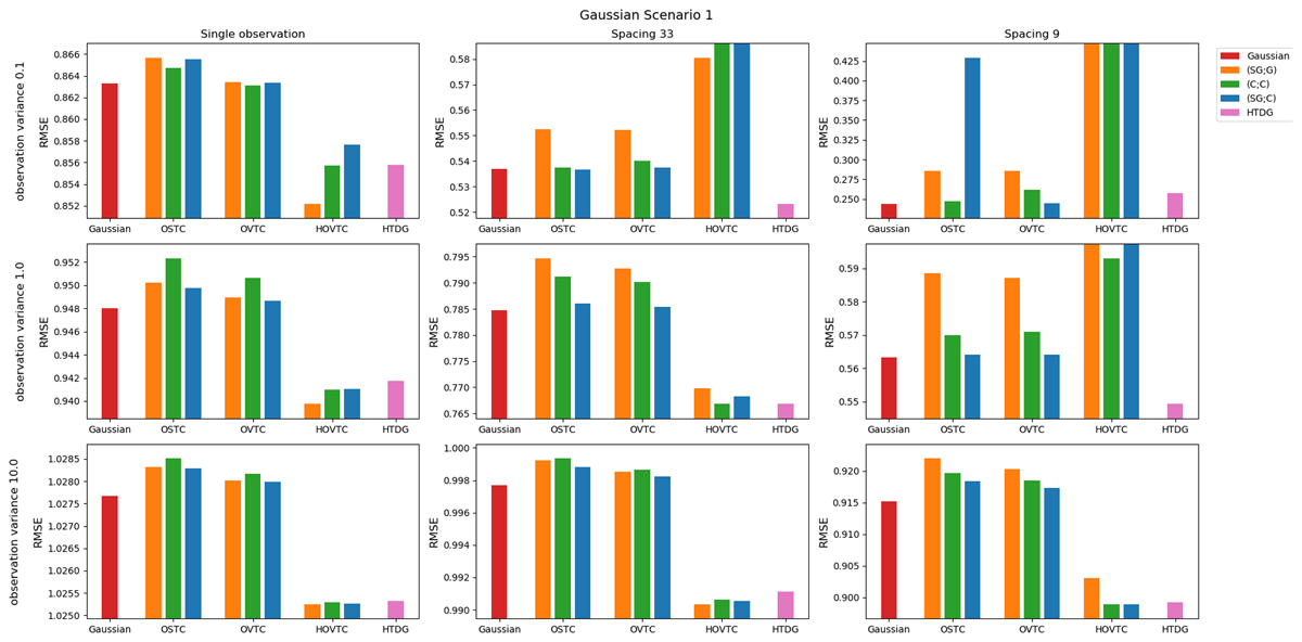
Figure 6
RMS errors resulting from DA with each kind of localisation in Gaussian Scenario 1. Columns show results for a range of observation spacing and rows show a range of observation error variance.
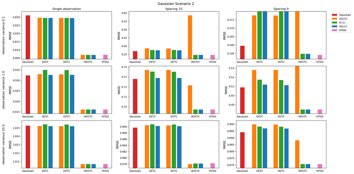
Figure 7
RMS errors resulting from DA with each kind of localisation in Gaussian Scenario 2. Columns show results for a range of observation spacing and rows show a range of observation error variance.