
1 Introduction
Numerical weather prediction (NWP) systems take an initial state and use dynamical models to evolve it forward in time to produce a forecast. A data assimilation (DA) process is then used to assimilate new observations into the forecast state to produce an initial state for the next forecast run. The exact state of the atmosphere is never known and the error statistics of the state and observations, in particular, the covariances, must be used to optimally combine the observations with the state. In ensemble methods, the covariance is estimated using the sample covariance of an ensemble of states. There is a need to mitigate the sampling error associated with this process, and this is often done using localisation, which damps the long range spurious correlations.
There are two types of errors associated with ensemble DA methods: the first occurs because the sampling process may have errors due to the states not being drawn from the true covariance matrix. The second type of error is sampling error, which results from the finite size of the ensemble. This can be explored using idealised models where the true distributions are known: this source of error is the focus of this paper.
Sampling error is a particular problem where the correlations between variables are small and the sampling noise can swamp the signal. Small correlations often occur at large physical distances and so a common problem is long range spurious correlations. Where they occur, the sample covariance contains erroneous large correlations between distant and weakly or unrelated variables in place of true small correlations. If unaddressed, erroneous large correlations can produce erroneous large increments that harm the analysis and forecast. This problem can be addressed by applying a localisation to the covariance matrix, which multiplies the sample covariance matrix element-wise by a matrix and cuts off or damps the correlations that are expected to be suffering from sampling noise (Houtekamer and Mitchell, 1998).
Many implementations use an ad-hoc tuning method to specify a localisation. They assume the correlations decrease with distance and, in order to mitigate the sampling error, either apply a cut off beyond which the correlations are zeroed (Houtekamer and Mitchell, 1998) or a damping to distant correlations (Houtekamer and Mitchell, 2001; Roh et al., 2015; Whitaker and Hamill, 2002). The shape of the damping is commonly a Gaspari-Cohn function which is similar to a Gaussian in shape but has compact support requiring it to go to zero at a finite distance (Gaspari and Cohn, 1999): it is identified by a width parameter. The width is tuned using past data and the shape is chosen to be similar to a Gaussian because the correlation tends to decrease with width. However, many shapes satisfy this assumption and there is nothing to suggest this particular choice is optimal. Additionally, there is no reason that the localisation width tuned initially would remain well tuned in time or be well tuned across a large area.
The aims of this paper are two-fold. First, is to develop a deeper understanding of ‘optimal localisations’ which optimise the accuracy of the analysis state. This includes exploring how different factors of the DA determine the optimal localisation and investigating the strengths/weaknesses of using different forms of localisation to optimise the analysis state. It is addressed by focusing on the single observation case where the optimal localisation of the gain can be derived. This is a step towards addressing the general case for any observation density which is extremely complicated. The second, parallel aim is to investigate the performance of derived localisations in the cases where they are not optimal. This includes identifying features of the optimal localisations that are valuable even when the deriving assumptions no-longer apply and using them to develop new tuneable localisations. All investigations take place in a simple, ideal model, representing a single variable state with known statistical behaviour.
Previous attempts have been made to investigate optimal localisation. They do not always optimise the analysis state. Ménétrier et al. (2015a) found the localisation that minimises the error between the true and localised sample covariance. This approach combined optimal linear filtering theory (analogous to OSTC presented in this paper) with centred moments estimation theory with the aim of expressing optimal filters in terms of statistics of the ensemble covariance and 4-order moment only. An ergodicity assumption is then used to evaluate the statistics, implying an averaging in space. Optimal localisations are identified that outperform traditional Gaussian approaches when their assumptions are met. Ménétrier et al. (2015b) applied this approach to an operational system and showed it can be used for successful DA, although there is a computational cost associated with the localisations computed at every DA step.
Perianez et al. (2014) found an expression for the optimal length scale of observation space localisation by minimising the analysis error, assumed to be made up of components due to the effective observation error and the approximation error. These experiments explored how observation density and observation error variance affected the optimal localisation length scale for a fixed localisation shape which is not necessarily optimal.
The work presented here builds on that by Flowerdew (2015) which uses a different approach to address state space localisation. It is assumed in Flowerdew (2015) and throughout this paper, that some climatological and sampling statistics are known, in addition to the ensemble of states, and these are used to evaluate the optimal localisation. This method produces static localisations for a climatology, implying an averaging over time (as opposed to spatial averaging imposed by Ménétrier et al. (2015a)). Flowerdew showed that the resulting localisations for a range of different covariance matrices were not Gaussian and can have a much more complex shape. Furthermore, this optimal localisation outperforms the best tuned Gaussian localisation in the cases considered.
Flowerdew (2015) focuses on optimising the gain, and not the covariance. This is because optimising the analysis relies on optimising the gain. When using the Kalman filter algorithm, using an optimal covariance localisation does not imply an optimal analysis because of the complex way the covariance (and its localisation) appear in the gain. The computation involves matrix multiplication, addition and inverse computation. This complexity also makes optimising the full gain extremely complex. Instead, a “sparse gain” for assimilating a single observation is optimised. The sparse gain localisation is applied to the covariance and remains optimal if the assumption holds that the sampling error in the variance is negligible. This paper follows the convention to optimise the sparse gain, building on it by investigating different application forms. Each computed localisation in this paper is implemented in three ways by, (i) applying the sparse gain localisation directly to the gain, (ii) applying the sparse gain localisation to the covariance and, (iii) applying the optimal covariance localisation directly to the covariance.
The localisation tested in Flowerdew (2015) is based on the assumption that there is a static, or known, true covariance matrix. Using the proposals outlined in Flowerdew (2015), this paper develops and tests two alternative “optimal” localisations derived under the assumption that the true covariance is not known, but a climatological distribution is known or predicted. One is a traditional localisation in which the localisation damps the sample covariance towards zero and the other is a hybridized localisation that damps the sample covariance towards the mean covariance. It is expected that this could produce analyses which better preserve the relationship between different but correlated assimilated variables. The development and testing of these methods is a fundamental step towards improving localisation schemes for more complex models including realistic weather models.
This paper extends the model used by Flowerdew to implement these two novel localisation methods and test their performance. The optimal localisations are scenario dependent and a Gaussian shaped covariance matrix model is used as the basis for the scenario following the work of Flowerdew (2015). The following objectives are addressed:
To incorporate a climatology into the model. This makes state and ensemble generation a two level process in which firstly a covariance is selected from the climatology, and secondly, states are selected from the covariance. This enables the statistics of the climatology to be used to compute optimal localisations.
To implement optimal localisation for a variable true covariance (OVTC) and a hybridized version (HOVTC) in a single observation scenario (in which the “optimal” status holds) and compare them to traditional Gaussian methods.
To investigate how increasing the density of the observations affects the performance of the computed localisations (OVTC and HOVTC) when the optimality no longer holds. This could provide insight into how the localisation should be adapted and applied for dense observations.
To investigate how the hybridized localisation (which damps towards a mean covariance not towards zero) compares to traditionally applied localisation. This includes testing if the hybridized version can be used to inform a tuned hybrid localisation (HTDG) with a comparable performance to Gaussian localisation.
The structure of the paper is as follows. In section 2, localisation methods are described. Section 2.1 describes the form of localisation schemes, section 2.2 describes where the localisation is applied and section 2.3 gives details of the sampling processes and the statistics needed to produce the optimal localisations. Section 3 describes the experimental framework with details about the model and the data assimilation application. Section 4 presents the results comparing the 3 types of localisation (i) traditional tuned Gaussian localisation (ii) theoretically derived localisations and (iii) a newly developed tuned hybrid localisation. Finally, section 5 provides a discussion of the findings.
2 Localisation Methods
2.1 Localisation types
In the experiments, an Ensemble Kalman Filter (EnKF) is used to perform the DA. Unlike other (e.g. variational) DA methods, the Kalman filter gives an explicit equation for the optimal update in terms of the covariance matrices. The covariance is directly computed and can be assessed and manipulated when using ensemble methods. It is, therefore, an ideal framework in which to attempt to extend the optimality to address the sampling error in the covariances, which occurs in ensemble methods. The Kalman Filter update equation is
where xa and xf are the analysis and (previous) forecast states respectively, K is the Kalman gain,
y is the vector of observations to be assimilated, Pf is the error covariance, R is the observation error covariance and h(∙) is the observation operator with linear approximation H. In the EnKF, the error covariance Pf is replaced with a localised sample covariance . This is traditionally of the form
where Lij is a localisation matrix applied by a Schur product to the sample error covariance matrix
which is computed from the N ensemble members xi and their mean. A localised Kalman gain, , is produced by using the localised sample covariance, , in place of Pf in equation (2). Alternatively, the sample gain, , computed using the sample error covariance, , in equation(2), can be localised directly
In ensemble methods the mean ensemble analysis state is found using
where the overbar represents the ensemble mean. Assessing the error in the mean analysis state avoids the related problems of addressing the spread in the analysis ensemble (or inflation) and focuses only on optimising and assessing the mean error in the ensemble DA. In the case with a single observation, y, taken at xi assimilated into point xj equations (1) and (2) become
where b is the sparse gain, σi is the standard deviation in the state error at i, rij is the correlation between the state error at points i and j and is the observation error variance at point j.
Table 1 summarises the 5 types of localisation considered in this paper. The Gaussian localisation is the traditional, form against which the new localisations are compared (Gaussian is used as opposed to Gaspari-Cohn localisation following previous work by Flowerdew, 2015). The OSTC has been applied in Flowerdew (2015). The application of the remaining 3 localisations (OVTC, HOVTC and HTDG) are novel to this paper.
Table 1
Types of Localisations. Bottom 3 rows show localisation application novel to this paper. Cost functions are given in terms of the parameter θ which represents the parameters of the distribution.
| LOCALISATION | COST FUNCTION | FORM | BASED ON |
| Gaussian | NA | Damps sample covariance towards 0. | Tuned width parameter γ. The distance between 2 points dij. |
| Optimal for a single covariance (OSTC) | Damps sample sparse gain towards 0. | Signal: (mean) sparse gain. Noise: mean variance in sample sparse gain. | |
| Optimal for a variable covariance (OVTC) | Damps sample sparse gain towards 0. | Signal: mean and variance in sparse gain. Noise: mean variance in sample sparse gain. | |
| hybrid Optimal for a variable covariance (HOVTC) | Damps sample sparse gain towards mean sparse gain. | Signal: variance in sparse gain. Noise: mean variance in sample sparse gain. | |
| hybrid tuned double Gaussian (HTDG) | NA | Damps sample covariance towards mean covariance. | Tuned width parameters γ1 and γ2. The distance between 2 points dij. |
All of the computed localisation factors can be expressed in terms of a signal to noise ratio, Q, as
Each computed localisation uses a different definition for the signal, as indicated in the final column of Table 1. In each case, the noise is the mean variance in the sample gain.
The first and last, Gaussian and hybrid tuned double Gaussian (HTDG), are both tuned using past data. The tuned parameters are found by running a suite of experiments for the given scenario for a range of values and selecting the one with the lowest RMS error. This process is an ad-hoc method and consequently is not expected to produce assimilation results that are optimally accurate.
The middle three localisations in Table 1: optimal for a single true covariance (OSTC), optimal for a variable true covariance (OVTC) and hybrid optimal for a variable true covariance (HOVTC), are all computed localisations given in terms of the sparse gain.1 They are optimal for assimilating a single observation, assuming there is no bias in the gain, and are derived in Flowerdew (2015) by minimising a cost function giving the squared distance between the localised sample gain and the true gain (i.e. the sparse gain calculated from the true covariance using equation (8).) Table 1 shows the cost function and resultant form of these three optimal localisations. OSTC gives the damping that is necessary to address the error due to sampling from a fixed covariance matrix, however, if the true covariance were known, there would be no need for ensemble methods or localisation. In a typical system, the covariance varies in time and its exact value is unknown at the assimilation step. However, a climatology describing a distribution of likely covariances may be estimated.
OVTC assumes there is a climatology specifying the variation in the true covariance and defines a theoretical optimal localisation to be applied to the sample sparse gain. HOVTC is an extension of the OVTC in which the localisation is applied to the variation of the sparse gain from its mean so as to provide an unbiased estimator of the gain:
where is the localised sparse gain, is the climatological mean sparse gain, is the ensemble sample sparse gain and α is a localisation factor. By preserving the mean gain, HOVTC is expected to produce localised gains that are closer to the true gain than the traditional forms which are damped towards zero. For multiple observations, hybrid localisation of the gain is applied as
where the damping is towards the mean sparse gain.2 HTDG is a tuned version of a hybrid localisation in which the localisation is applied such that the localisation damps towards the mean covariance,
Its shape is composed of two Gaussians and has been chosen to be a similar shape to the optimal hybrid localisation in the experiments (see Section 4 for more details).
2.2 Localisation Application
The optimal localisations: OSTC, OVTC and HOVTC, are derived to be optimal when assimilating a single observation. When they are applied to cases with multiple observations they are referred to as computed localisations. Each localisation in this paper is implemented in three ways by, (i) applying the sparse gain localisation directly to the gain, (SG;G). (ii) applying the optimal covariance localisation directly to the covariance (C;C) and, (iii) applying the sparse gain localisation to the covariance (SG;C).
The first application is where the sparse gain computed localisation is applied directly to the gain (SG;G). The localisation factors given in Table 1 are expressed and applied to a sparse gain, b. In multiple observation cases, the sparse gain localisation is applied to the multiple observation gain.
Optimal covariance localisations, (C;C) can be found by replacing the sparse gain, b, with the covariance Pf in the cost functions and localisation factors given in Table 1. This produces the most accurate covariance from the sample covariance using equation (3) or equation (12) but it does not necessarily optimise the analysis. In the limit that the covariance is accurate, the true covariance produces the true gain. However, sampling errors in the covariance become sampling errors in the gain via equation (2) (or equation (8) for the sparse case). This transformation is complex involving a matrix inverse (or ratio of correlated sampling errors). Therefore, addressing the sampling error that occurs in the covariance (in a way that optimises the analysis) needs to take into account how the errors propagate through the gain.
The final application type is to apply the sparse gain localisation to the covariance (SG;C). To achieve this, a representative observation error variance, , is assigned to points without an observation. The same observation error variance is used for all observations in each experiment, and for all unobserved points. This enables the sparse gain (equation (8)) and its statistics to be computed for every pair of grid points, and ensures the statistics are continuous across both observed and unobserved points.
In the single observation case, applying any of the optimal localisations of the sparse gain to the gain is equivalent to applying it to the covariance if two assumptions hold. Firstly, that there is no climatological variation in the variances, and secondly, that there is no sampling error in the sample variances . The experiments in this paper have static variances so the first assumption holds. The standard deviation in the sample variance of size N taken from a normal distribution N(μ, σ2) with mean μ and variance σ is (Casella and Berger, 2002, example 7.3.3, p. 331)
which indicates the variance is small for ensemble size 10 but not zero, so the second assumption does not strictly hold but can be approximated.
It is interesting to explore this application type because, although the (SG;G) localisations are optimal, implementations of equation (5) or equation (10) for a single observation, they apply no localisation in the inverse matrix term, , of the gain. A localisation applied to the covariance, on the other hand, addresses the sampling error at source. For a single observation, only the variance is not localised in the denominator of the sparse gain, but for multiple observations, more terms are not localised. Complex effects also occur when assimilating multiple observations. It is known that observations interact and can reinforce each other (Lorenc 1981, Bannister 2008). This is a reason to apply the localisation to the covariance before the spurious correlations could cause additional effects in the assimilation through “reinforcing” effects in the gain. Covariance localisation (SG;C) may therefore be expected to be similar to the gain localisation (SG;G) for sparse observations and be more robust to dense observations. However, the (SG;C) localisation does not optimise the DA or the covariance.
2.3 Sampling processes and computed statistics
A two layered sampling process is used to specify the sampling of states from the climatology. The climatology is referred to as a Scenario and is defined as a distribution of covariance matrices. A Scenario describes the longer term variability in the weather. Sampling from a Scenario produces a covariance matrix referred to in this paper as a Regime. A Regime describes the variation in the states of an ensemble and can be thought of as the uncertainty on a shorter scale e.g. a day. Sampling from a Regime produces States: ensemble and truth states are all sampled from the same Regime. Finally, a State is a single value of every parameter at every point which can be thought of as representing a possible state at a moment in time.
Statistics needed to calculate the localisations are computed by empirically drawing covariances from the Scenario and states from the Scenario and Regime, converting them to sparse gains via equation (8) and taking appropriate statistics. Specifically, to obtain the mean and variance of the gain, a large number (10000) of Regime covariances are generated from the Scenario and converted to sparse gains. The mean and variance of these are then computed.
For gain localisations (SG, G, SG; C), the mean variance in the sample gain, , is computed by a three step process. First a range of Regimes is sampled from across the climatology (1000 samples). For each Regime a large number (1000) of sample sparse gains calculated from ensembles of size 10 can be computed and from them, the variance is computed. Finally, the mean is taken of the variances over the different Regimes. Similar processes are used to compute the statistics of the covariance for optimal covariance localisations, (C;C).
OVTC and HOVTC localisations are defined in terms of a climatology but OSTC is not, as it is based on the assumption of an underlying static true covariance. Where OSTC is applied, the mean sparse gain/covariance is used as the true gain/covariance and the mean variation in the sample sparse gain/covariance is used as the variation in the sample gain/covariance.
3 Experimental Framework
Python 3.7 was used to develop an object-oriented package of code to perform the localisation experiments.
In the experiments, a State gives the value of a single variable on a one-dimensional domain of grid points. A Regime is specified as the correlation between points given by a Gaussian shaped covariance matrix
where dij is the distance between grid points i and j and γ is a specified width parameter. Sampling from a Regime to produce States is done via eigenvector decomposition. The climatology (a Scenario) can be thought of physically as an expectation that the weather will exist on a range of spatial scales. It is represented as a uniform distribution of the width parameter, γ between two boundary values (e.g. between 5 and 40).
A number of additional parameters were set via a series of initial experiments and fixed for all subsequent experiments. The number of ensemble members was set at 10 as this was small enough to show the effects of sampling error. The number of times the experiment was repeated was fixed at 100,000. This was large enough to produce reliable RMS analysis error results whose relative ordering did not change when the experiments were repeated. The number of grid points was fixed at 100 to keep the computational cost of the model down. The Scenario scale and observation density were chosen relative to the number of grid points so that the detail of the Scenario’s form, and the impact of different density regimes could be investigated. The observation error covariance was assumed to have independent cross correlations (set to zero) as this was the simplest case and a common assumption operationally. The observation error variance was set to 0.1, 1.0 or 10.0 (low, medium or high) indicating the assimilation strength was respectively strong, equal or weak as the true background error variance implied by equation (14) is 1.
Three schematic figures show how the code functions to produce the results. Figure 1 shows the process of assimilating a single (set of) observation(s) into a forecast ensemble to produce an analysis state. Figure 2 summarises the process of performing a single DA cycle where a Scenario is specified and used to generate the analysis state and RMS errors in the analysis state are computed to give a measure of the DAs performance. Figure 3 shows the highest structure level of the experiments which produce results that average over a large number of individual DA cycles.
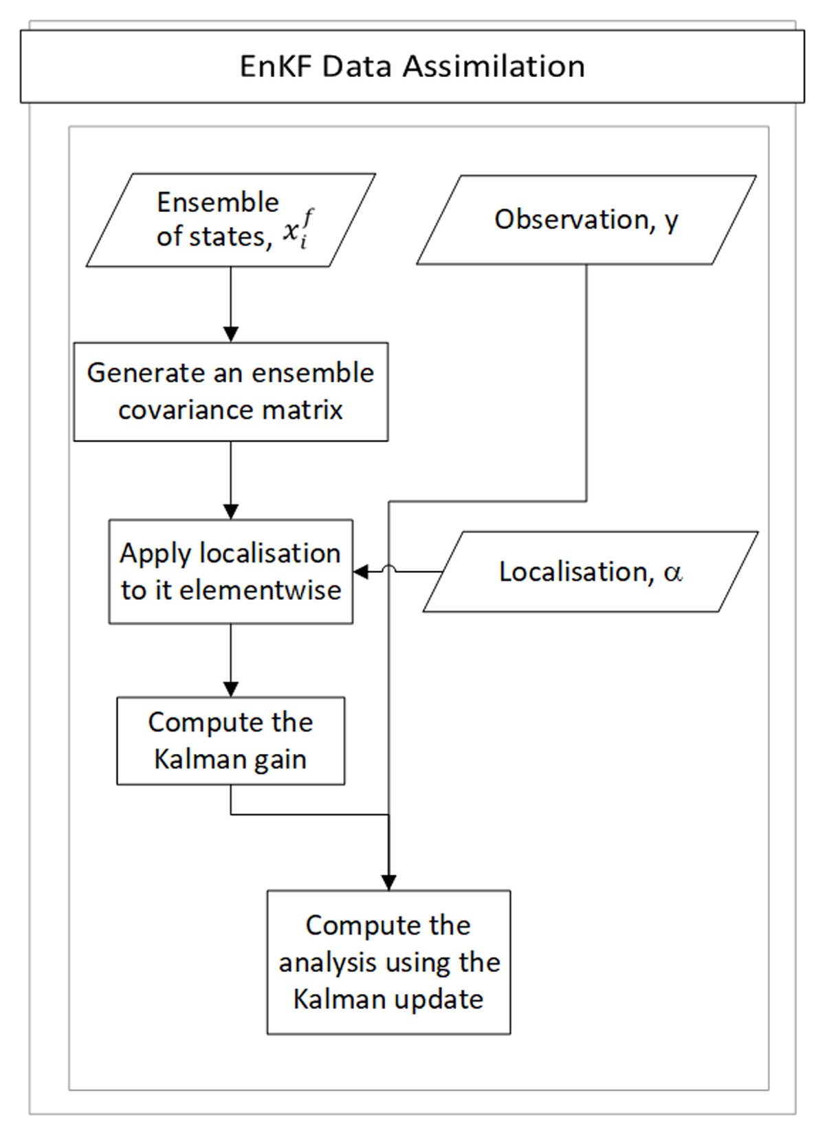
Figure 1
Schematic of a single DA process using the EnKF.
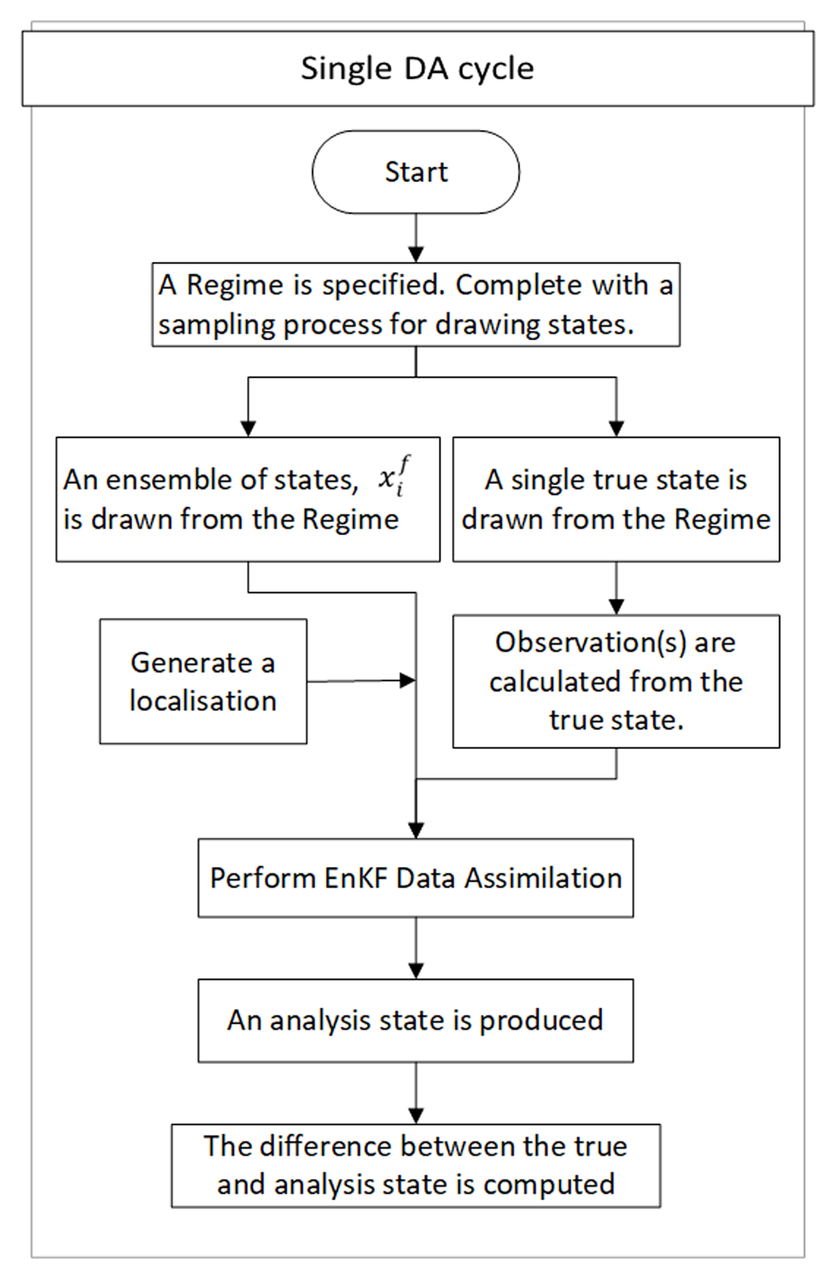
Figure 2
Schematic showing the ensemble and observation generation, assimilation and error production for a single DA cycle.
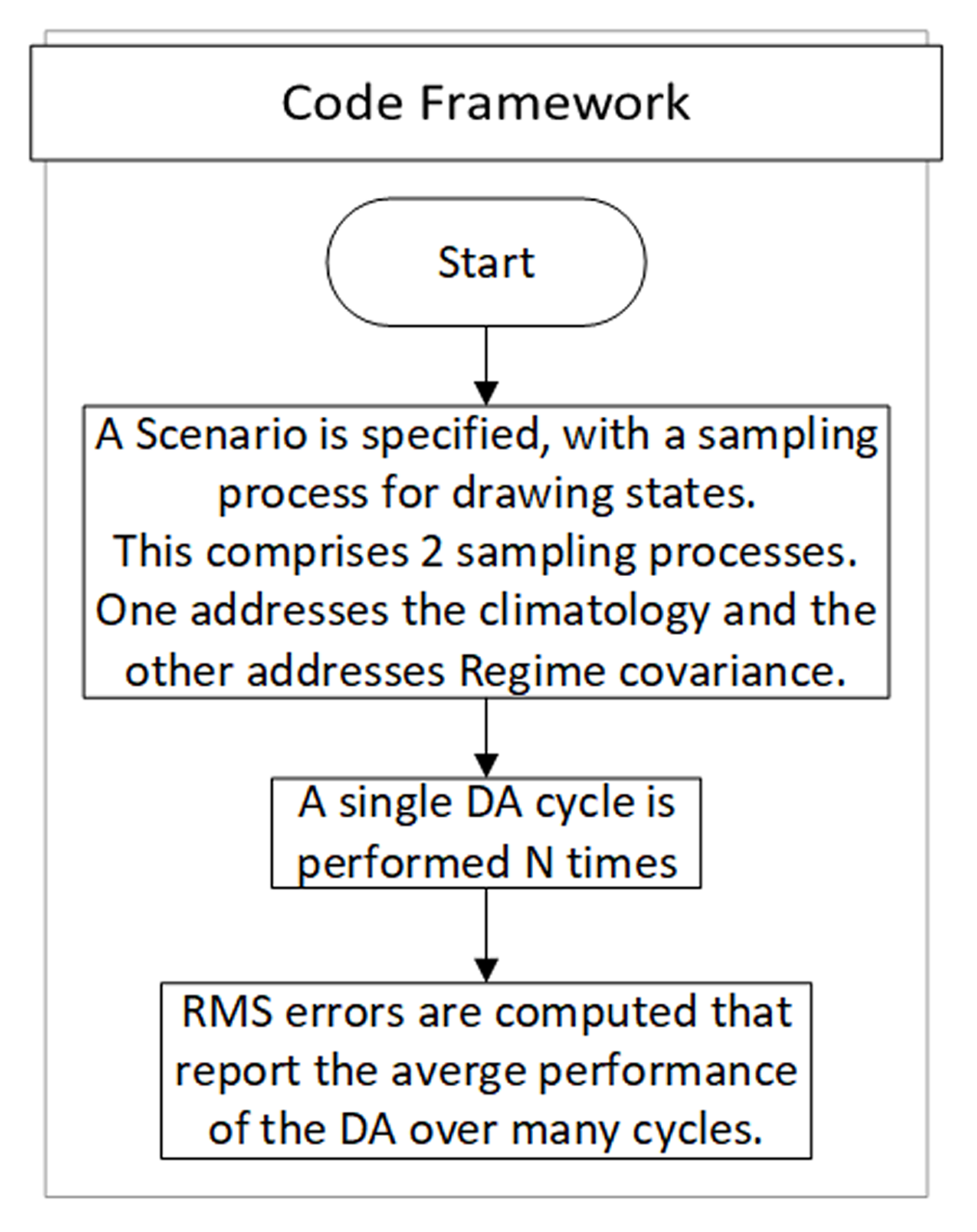
Figure 3
The flow diagram of the experiments performed and reported in this paper.
4 Comparison of Localisations and their Performance
A suite of experiments investigating the Gaussian Scenario with width parameter uniformly distributed between 5 and 40 were performed (Scenario 1). These experiments were repeated for 3 observation error variances namely 0.1 (strong assimilation), 1.0 (equal strength assimilation) and 10.0 (weak assimilation) and for 3 observation densities. The observation densities were: (i) a single (sparse) observation; (ii) regularly spaced (medium) observations with large spacing of 33 grid points between observations (equivalent to 4 observations across the domain) and (iii) small spaced (dense) observations with 9 grid points between observations (equivalent to 12 observations across the domain).
A second suite of runs were then performed for the same Gaussian Scenario with the width parameter uniformly distributed between 20 and 30 (Scenario 2) to explore the impact of the variability in the climatology.
4.1 Signal, noise and localisation factors
Figure 4 shows the form of the localisations applied in the single observation experiment for each assimilation strength in Scenario 1. The first row of plots shows the statistics that are used to construct the computed localisations. The mean gain and the variance in the gain are used to construct the signal in the computed gain localisation ( see Table 1 for how the signal is constructed for each localisation). The square root of the mean variance in the sample gain represents the noise. This is also plotted with the error in the variances replaced with the true background error variance (one). This statistic is the scaled square root mean variance in the correlation: it represents the noise term in the gain due only to the sampling error in the correlation. The scaled square root of the mean variance in the sample covariance shows the behaviour of the noise term in the (C;C) localisations. The covariance statistics are scaled by dividing by the expected denominator of the sparse gain, (). Finally, the mean sample gain is shown. This differs from the mean gain indicating that there is some bias in the gain and the bias is worst for the case with observation error variance 1.0.
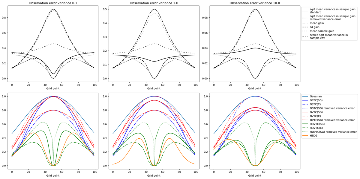
Figure 4
Plot showing the shape of each localisation and the statistics used to compute the localisation for Scenario 1. The form of the localisations is shown for observation variance 0.1, 1.0 and 10.0. The shown tuned widths are tuned from assimilating a single observation.
The second row of plots shows the resultant form of the computed localisation types for optimising the gain, the covariance, and the gain with variance errors removed (equivalent to optimizing the correlation and neglecting sampling error in the variance). Also shown is the form of the tuned Gaussian and HTDG localisation used for the single observation case.
It can be seen that for strong assimilation (observation error variance 0.1) the sparse gain noise and localisations behave similarly to the case with the removed variance error. This is because for small observation error variance, the sample gain behaves as
so that, where the sampling error in and are correlated, their sampling errors approximately cancel. An expression can be found for the covariance between the sampling error in the variances (Raynaud et al., 2009)
which shows the correlation between the sampling error in the variances is proportional to the square of the true correlation rij. This implies that where the sampling error in and are uncorrelated, the correlation rij is small. This implies the sampling error in the correlation rij is large and the sampling error in the sparse gain is dominated by the sampling error in the correlation rij. For weak assimilation (observation error variance 10.0), the sparse gain noise and localisation behave more similarly to the covariance. This is because the observation error variance dominates the denominator of the sparse gain and the sampling error in the sparse gain is dominated by the sampling error in the numerator i.e. the covariance. In the equal assimilation case, the behaviour of the sparse gain statistics and localisation lies between the case with removed variances and the covariance case.
The Gaussian localisation peaks at 1 but the optimal localisations of the gain, peak at less than 1 which implies that they damp the update even at the observed point. This is due to the non-vanishing sampling error in the sample gain. The first case with observation variance 0.1 is the only case with near unit localisation applied to the update at the observed point. The OSTC and OVTC localisations agree at the peak but the OVTC allows more signal through at intermediate distances as is indicated by the broader OVTC curve compared with the OSTC curve. This is because OVTC allows for more variability in the true gain/covariance due to the climatology.
When studying the hybrid localisations (optimal and tuned), it is important to note that they are localising the departure from the mean covariance and not the covariance. Therefore, where the hybrid localisation is zero, this does not correspond to zeroing the covariance or gain matrix but instead to using its climatological average. The hybrid localisation for this Scenario has two peaks either side of the zeroed centre. The tuned hybrid localisation, HTDG, was constructed from 2 Gaussians to have a similar double peaked shape to the optimal hybrid localisation. The equation for its form is given in Table 1 and is given in terms of 2 width parameters to tune. HTDG was tuned separately for each observation density and assimilation strength.
A similar plot for Scenario 2 is shown in Figure 5. A key difference between the Scenarios is the standard deviation in the gain which is much smaller in Scenario 2. This causes OSTC and OVTC to be similar as the assumption of OSTC that the true covariance is static is a more reasonable approximation. For HOVTC, the small amount of variability in Gaussian Scenario 2 and the hybrid structure allows it to identify that the ensemble covariance/gain is always close to the climatological mean covariance/gain. The HOVTC localisation factor is small and the adjustment made to the mean covariance using the ensemble data is small. In Gaussian Scenario 1 the HOVTC localisation makes a much larger adjustment to the mean covariance/gain due to the large amount of variability in the Scenario. The effect of the variability of the Scenario on the form of the traditionally applied localisation is less significant because of the inclusion of the mean gain/covariance in the signal. This means, at intermediate distances where the variability is most significant in this Scenario, the mean gain/covariance is still a significant component of the signal determining the form of the localisation.
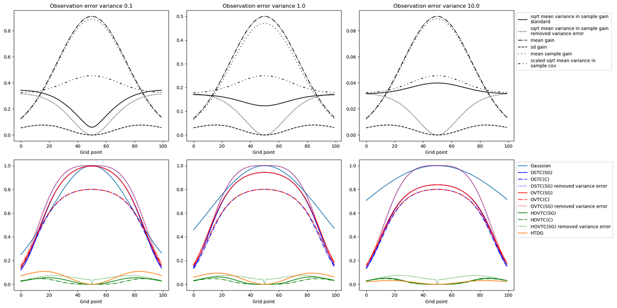
Figure 5
Plot showing the shape of each localisation and the statistics used to compute the localisation for Scenario 2. The form of the localisations is shown for observation variance 0.1,1.0 and 10.0. The shown tuned widths are tuned from assimilating a single observation.
4.2 Analysis Error Results
Table 2 shows the overall RMS analysis error results for experiments using Scenario 1, comparing localisation performance for various observation spacing and observation error variance. The RMS error between the true state and the assimilated state produced by the experiment is given for each localisation type. To put these results in context, the background error, computed as the RMS error between the ensemble mean and the true state averaged across the regime, is approximately 1.046 in every experiment.3 The difference between the background error and localised error, therefore, indicates the error improvement made by the assimilation process. These results are plotted in Figure 6. Similarly, Table 3 shows the results for Gaussian Scenario 2 which are plotted in Figure 7. Note that where the bars go off the top of the chart, in both figures, the error is greater than the background error.
Table 2
RMS error results for Scenario 1.
| SCENARIO 1 OBSERVATION ERROR VARIANCE 0.1 | ||||||||||||
|---|---|---|---|---|---|---|---|---|---|---|---|---|
| OSTC | OVTC | HOVTC | ||||||||||
| GAUSSIAN | (SG;G) | (C;C) | (SG;C) | (SG;G) | (C;C) | (SG;C) | (SG;G) | (C;C) | (SG;C) | HTDG | BACKGROUND ERROR | |
| Single ob | 0.8633 | 0.8656 | 0.8647 | 0.8656 | 0.8634 | 0.8631 | 0.8633 | 0.8522 | 0.8557 | 0.8576 | 0.8558 | 1.0466 |
| Spacing 33 | 0.5368 | 0.5525 | 0.5376 | 0.5366 | 0.5523 | 0.5402 | 0.5375 | 0.5804 | 2.4186 | 14.7818 | 0.5233 | 1.0462 |
| Spacing 9 | 0.2440 | 0.2852 | 0.2468 | 0.4289 | 0.2855 | 0.2613 | 0.2449 | 1.8869 | 212.2495 | 38.626 | 0.2573 | 1.0461 |
| SCENARIO 1 OBSERVATION ERROR VARIANCE 1.0 | ||||||||||||
| OSTC | OVTC | HOVTC | ||||||||||
| GAUSSIAN | (SG;G) | (C;C) | (SG;C) | (SG;G) | (C;C) | (SG;C) | (SG;G) | (C;C) | (SG;C) | HTDG | BACKGROUND ERROR | |
| Single ob | 0.9480 | 0.9502 | 0.9523 | 0.9498 | 0.9490 | 0.9506 | 0.9487 | 0.9398 | 0.9410 | 0.9411 | 0.9417 | 1.0466 |
| Spacing 33 | 0.7848 | 0.7947 | 0.7911 | 0.7860 | 0.7927 | 0.7901 | 0.7854 | 0.7698 | 0.7668 | 0.7682 | 0.7669 | 1.0462 |
| Spacing 9 | 0.5633 | 0.5886 | 0.5701 | 0.5641 | 0.5870 | 0.5709 | 0.5642 | 1.1460 | 0.5931 | 4.6481 | 0.5493 | 1.0461 |
| SCENARIO 1 OBSERVATION ERROR VARIANCE 10.0 | ||||||||||||
| OSTC | OVTC | HOVTC | ||||||||||
| GAUSSIAN | (SG;G) | (C;C) | (SG;C) | (SG;G) | (C;C) | (SG;C) | (SG;G) | (C;C) | (SG;C) | HTDG | BACKGROUND ERROR | |
| Single ob | 1.0277 | 1.0283 | 1.0285 | 1.0283 | 1.0280 | 1.0282 | 1.0280 | 1.0252 | 1.0253 | 1.0253 | 1.0253 | 1.0466 |
| Spacing 33 | 0.9977 | 0.9992 | 0.9993 | 0.9988 | 0.9985 | 0.9987 | 0.9982 | 0.9903 | 0.9906 | 0.9906 | 0.9911 | 1.0462 |
| Spacing 9 | 0.9152 | 0.9220 | 0.9197 | 0.9184 | 0.9203 | 0.9184 | 0.9173 | 0.9031 | 0.8989 | 0.8989 | 0.8992 | 1.0461 |
Table 3
RMS error results for Scenario 2.
| SCENARIO 2 OBSERVATION ERROR VARIANCE 0.1 | ||||||||||||
|---|---|---|---|---|---|---|---|---|---|---|---|---|
| OSTC | OVTC | HOVTC | ||||||||||
| GAUSSIAN | (SG;G) | (C;C) | (SG;C) | (SG;G) | (C;C) | (SG;C) | (SG;G) | (C;C) | (SG;C) | HTDG | BACKGROUND ERROR | |
| Single ob | 0.8311 | 0.8296 | 0.8295 | 0.8295 | 0.8295 | 0.8295 | 0.8294 | 0.8068 | 0.8068 | 0.8068 | 0.8070 | 1.0469 |
| Spacing 33 | 0.3701 | 0.3858 | 0.3763 | 0.3745 | 0.3856 | 0.3758 | 0.3739 | 0.5856 | 0.3495 | 0.3460 | 0.3459 | 1.0464 |
| Spacing 9 | 0.1995 | 0.2175 | 152.6382 | 136.7548 | 0.2174 | 16.2293 | 109.381 | 3.4972 | 0.1947 | 0.1947 | 0.1940 | 1.0463 |
| SCENARIO 2 OBSERVATION ERROR VARIANCE 1.0 | ||||||||||||
| OSTC | OVTC | HOVTC | ||||||||||
| GAUSSIAN | (SG;G) | (C;C) | (SG;C) | (SG;G) | (C;C) | (SG;C) | (SG;G) | (C;C) | (SG;C) | HTDG | BACKGROUND ERROR | |
| Single ob | 0.9324 | 0.9329 | 0.9350 | 0.9326 | 0.9329 | 0.2349 | 0.9326 | 0.9161 | 0.9161 | 0.9161 | 0.9161 | 1.0469 |
| Spacing 33 | 0.7279 | 0.7370 | 0.7352 | 0.7289 | 0.7370 | 0.7352 | 0.7288 | 0.7215 | 0.6971 | 0.6971 | 0.6971 | 1.0464 |
| Spacing 9 | 0.5089 | 0.5280 | 0.5173 | 0.5119 | 0.5280 | 0.5170 | 0.5113 | 1.8282 | 0.4846 | 0.4846 | 0.4847 | 1.0463 |
| SCENARIO 2 OBSERVATION ERROR VARIANCE 10.0 | ||||||||||||
| OSTC | OVTC | HOVTC | ||||||||||
| GAUSSIAN | (SG;G) | (C;C) | (SG;C) | (SG;G) | (C;C) | (SG;C) | (SG;G) | (C;C) | (SG;C) | HTDG | BACKGROUND ERROR | |
| Single ob | 1.0253 | 1.0252 | 0.0254 | 1.0252 | 1.0252 | 1.0254 | 1.0252 | 1.0207 | 1.0207 | 1.0207 | 1.0207 | 1.0469 |
| Spacing 33 | 0.9897 | 0.9904 | 0.9907 | 0.9902 | 0.9904 | 0.9907 | 0.9901 | 0.9780 | 0.9782 | 0.9782 | 0.9782 | 1.0464 |
| Spacing 9 | 0.8941 | 0.8998 | 0.8982 | 0.8969 | 0.8997 | 0.8982 | 0.8968 | 0.8882 | 0.8706 | 0.8706 | 0.8707 | 1.0463 |
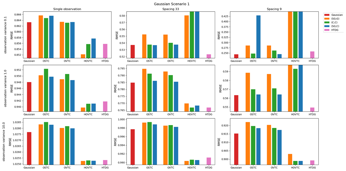
Figure 6
RMS errors resulting from DA with each kind of localisation in Gaussian Scenario 1. Columns show results for a range of observation spacing and rows show a range of observation error variance.
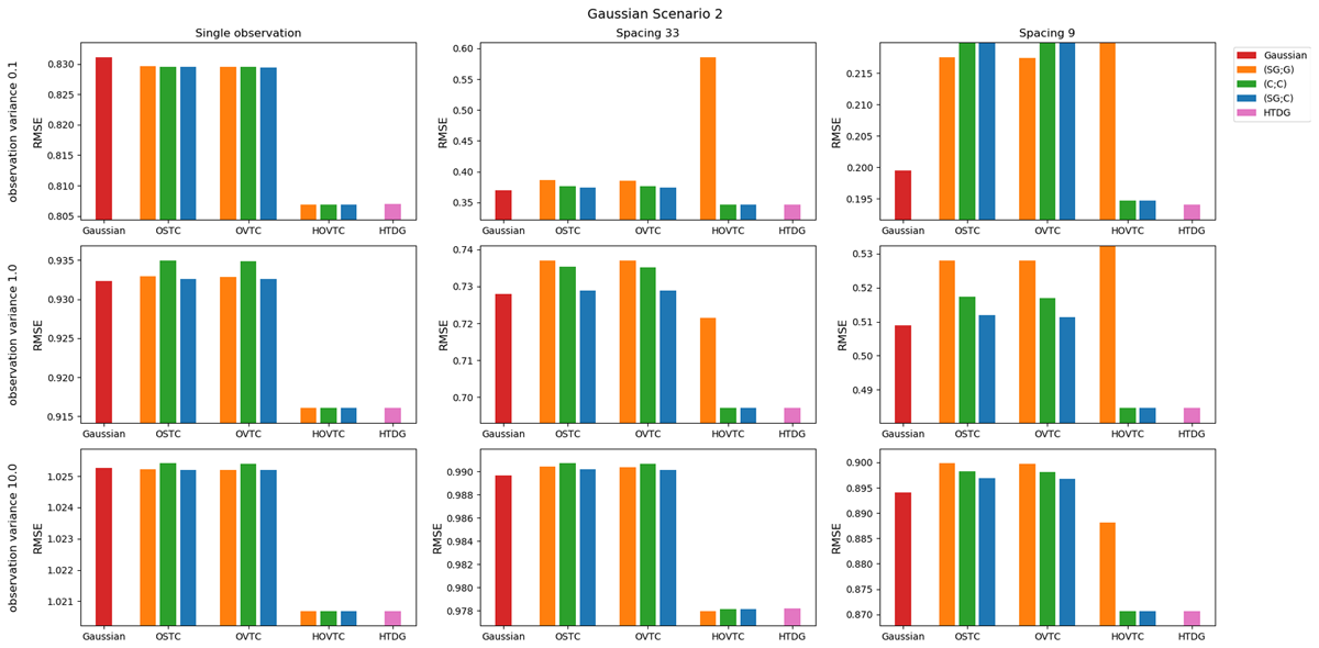
Figure 7
RMS errors resulting from DA with each kind of localisation in Gaussian Scenario 2. Columns show results for a range of observation spacing and rows show a range of observation error variance.
Common patterns and interesting results from both suites of results are discussed. The term ‘effective observation density’ is used to refer to the density in the context of the other properties of the case. A high effective observation density implies that there are a lot of observations that have a significant impact on the update at a point. Specifically, the effective observation density is high if cross covariances occur in the inverse matrix, , of the gain which have a significant impact in determining the form of the gain. The number of observations, assimilation strength and Scenario all affect it. Increasing the assimilation strength increases the effective observation density as the smaller observation error variance means the sample covariance terms, in the inverse matrix of the gain, play a larger role in determining its magnitude. Increasing the number of observations increases the effective observation density by causing more sample covariance terms to occur in the inverse matrix of the gain. Similarly, if the Gaussian Scenario contains (on average) larger widths (γ), then this implies more significant correlations. The observation effects will be less separable, which therefore implies a larger effective observation density.
Single Observation Experiment
First, we consider the single observation cases where the computed (SG;G) localisations are expected to be optimal. In all experiments assimilating a single observation, the best performing computed localisation type, for any given application type, is HOVTC followed by OVTC which outperforms OSTC. The climatologically aware computed localisations perform better than OSTC which assumes a static true covariance matrix. The optimal hybrid form of localisation performs better than the optimal traditionally applied localisation. This ordering of results also occurs in some multiple observation cases where the effective observation density is low enough that optimality is still approximated by the computed localisations. However, when the effective observation density is too high, the computed localisation can perform poorly and this order can reverse.
In the single observation case, OVTC(SG;G) might be expected to be the best performing traditionally applied localisation as it optimises the gain; however this is not observed. Results show that OSTC(SG;C) performs equally as well as OVTC(SG;G) and in many cases better than it. This is because a localisation of the covariance can apply localisation more directly in all places throughout the gain. Specifically, it addresses the sampling error in the inverse matrix of the gain (in the single observation case to the variances) which cannot be addressed when applying localisation directly to the gain. In the strong assimilation cases, optimal localisation of the gain behaves similarly to optimal localisation of the correlation meaning OVTC(C;C) can have the advantage in addressing the sampling error in the variance in the denominator of the gain and is the best performing localisation for Scenario 1. However, for equal and weak assimilation the OVTC(SG;C) has the advantage over OSTC(C;C) because the correlations in the sampling error in the gain mean that the optimal covariance localisation does not approximate optimising the gain and applying the optimal gain localisation to the covariance applies localisation in the numerator of the gain that addresses these correlations whilst still applying some damping to the sampling error in the variance in the denominator of the gain. In Scenario 1 the Gaussian outperforms OVTC(SG;G). This cannot be explained by variance localisation in the denominator as the Gaussian applies a localisation factor of 1 to the variances. It has been shown that the sparse gain is biased towards zero, which can explain why OVTC is slightly sub-optimal and the Gaussian is able to perform better than it. OVTC(SG;G) performs similarly to the best tuned Gaussian in all cases and is most significantly outperformed by the Gaussian in the equal assimilation case where the bias in the gain is greatest. The success of the Gaussian shows it is an appropriate tuneable shape for this Scenario.
For assimilating a single observation, HOVTC(SG;G), which is expected to be optimal, is the best performing localisation in every experiment (even in the cases where there is a known bias in the gain). HOVTC(C;C) produces lower analysis errors than HOVTC(SG;C). This is, in part, due to the effectiveness of hybridizing the covariance which enables the true covariance to be better represented across the whole domain. The difference between HOVTC(SG;G) and HOVTC(SG;C) is also more significant than for traditionally applied localisations. They are still approximately equivalent if the sampling error in the variance is negligible, however, the construction of the hybrid localisation means that the mean gain is no longer part of the signal. Therefore, there is a finer balance between the noise and signal and the sampling error in the variance has a greater impact on the overall hybrid localisation factor and behaviour. HTDG performs better than the traditionally applied localisations and similarly to, but not better than, the HOVTC localisations in the single observation case.
Overall, in the single observation cases, the climatologically aware traditionally applied OVTC localisations perform similarly to the Gaussian. They do not perform reliably better because the sparse gain has been shown to be biased causing OVTC to be suboptimal. Also localising the sparse gain directly can be less desirable than localising the sampling error at source in the covariance. The HOVTC outperforms all the traditionally applied localisations. This shows that applying a hybrid localisation can improve upon traditionally applied localisations that damps the sample gain/covariance matrix towards zero.
Multiple Observation Experiments
For experiments with multiple observations assimilated, the computed localisations are not optimal and sometimes produce extreme analysis errors greater than the background errors. Where the effective observation density is low enough, they can still produce good results. For traditionally applied, computed localisations, with low or intermediate effective observation density, it is common for (SG;G) application types to be outperformed by both the (C;C) and (SG;C) application. This is because applying a localisation to the covariance is desirable for multiple observation cases as more terms with sampling error occur in the inverse matrix of the gain and benefit from being localised directly. It is also common for the covariance (C;C) application types to be outperformed by (SG;C). This is because in (SG;C), the sparse gain localisation is applied to the covariance in the inverse matrix of the gain, so the sampling error that occurs there is damped. Meanwhile, it can also address properties that arise from the behaviour of the sampling error correlations in the gain due to its application in the numerator of the gain. For a high enough effective observation density, all the computed localisations are sub-optimal and may break down producing extreme results.
The traditionally applied optimal covariance localisation OVTC(C;C) breaks down and produces extreme analysis errors for the highest effective observation density case in Scenario 2, (strong assimilation, spacing 9). This is important, because it is an example of the possible pitfalls of the commonly attempted approach of finding a localisation that optimises the covariance directly. Specifically, it shows that optimising the covariance (C;C) can be highly different to optimising the gain or analysis state.
The behaviour of the application types of HOVTC for multiple observations is different. For intermediate effective observation density, HOVTC(C;C) tends to outperform HOVTC(SG;C) and HOVTC(SG;G) (which was not observed for OVTC). The success of HOVTC(C;C) implies that the hybridised localisation of the covariance enables a significant improvement in the accurate representation of the true covariance which leads to a more accurate gain. The (SG;C) form performs less well, because the finer balance between the signal and noise in HOVTC, means that the sampling error in the variances play a more significant role in determining the localisation factor. This means that the difference between the optimal localisation of the covariance and of the gain is larger in a hybrid localisation compared with a traditional one and the penalty for applying the localisation differently from how it is derived is greater. For high enough effective observation density, all the computed localisations can break down.
The variability of the climatology, and whether the localisation is hybrid or traditionally applied, impacts on the ability of the localisation to represent the truth and hence the performance of the computed localisations. The small amount of variability in Scenario 2 means that OSTC and OVTC are very similar. In this case, the assumption of OSTC that the true covariance is static is a reasonable approximation. However, for Gaussian Scenario 1, with more variability in the Regime, OVTC has a significant advantage over OSTC. In Scenario 1, HOVTC localisations break down for the highest density cases but they do not in Scenario 2 where the mean covariance is closer to the true covariances and not adjusted much by the ensemble.
In almost every case considered, for single and multiple observation cases, the best performing localisation was a hybrid localisation (either HOVTC or HTDG). This shows the effectiveness of the proposed hybrid form of localisation. Its advantage is in separating out the mean gain/covariance which enables the finer balance between the signal, due to the climatological variability about the mean gain/covariance, and the noise to be addressed. The traditionally applied localisations can only damp the noise at the expense of damping the mean gain/covariance. The Gaussian outperforms all hybrid localisations in one case: the strong assimilation case with the highest observation density (observation spacing 9) in Scenario 1. This is because, for high observation density, overdamping the intermediate correlations is rewarded as making the best use of local information outweighs the benefits of preserving the mean.
The HTDG results show analysis errors closer to the HOVTC for single observations than any of the traditionally applied localisations. For denser observations, HTDG was retuned and was able to adapt to denser regimes and be the best performing localisation where HOVTC breaks down. This is therefore an example of developing an effective tuneable hybrid localisation inspired by the form of the optimal localisation for a single observation.
5 Discussion
This paper has assessed the performance of optimally derived localisations to address the sampling error in the EnKF when performing DA for a model based on Gaussian shaped covariances. It addresses two related goals. First, to investigate what the optimal localisation is and what affects it. This was demonstrated through the single observation case, where the Kalman gain was simple enough for an optimal gain localisation to be derived. The second goal was to advance insight into the dense observation cases and propose how knowledge about optimal localisation in the sparse case, may be used to inform better localisation methods for the dense case without knowing the full optimal solution.
A number of aspects of the DA have been shown to be important in determining the optimal localisation. These include the localisation application (applied to the covariance or gain) and type (traditional or hybrid damping), the Scenario including the variability of its climatology, the assimilation strength and the observation density.
Three localisation application types (SG;G), (C;C) and (SG;C) were explored. It is desirable to optimise the analysis state, however that is complex. It is therefore more common to directly optimise the covariance, (C;C). One novel aspect of this paper is that it has attempted to optimise the analysis state via optimising the direct localisation of the Kalman gain in the sparse (single) observation case, (SG;G). Here, it should be noted that direct localisation of the gain does not apply any localisation directly to the sampling error in the inverse matrix of the gain which does occur when applied to the covariance. It was seen that in the intermediate density cases, (SG;C) which applies the localisation derived for the sparse gain to the covariances, performed better than (C;C). (SG:C) has properties of a sparse gain localisation but also applies some damping in the inverse matrix of the gain. This emphasises that it would be most desirable to optimize the full Kalman gain with localisation applied to the covariance, however, the complexity of that problem is a significant deterrent. An optimal localisation of the full Kalman gain would have to take into account the behaviour of the cross correlations occurring in the inverse matrix of the gain. It’s possible that applying a different localisation in the PHT and the inverse matrix, , of the gain could also be beneficial as the roles played by the covariance in each are different. A possible future first step to investigate such a scheme would be to attempt to optimize the sparse gain with 2 localisation factors: one multiplying just the covariances in the denominator of the gain and one multiplying the whole gain.
A second choice made when designing a localisation scheme is the type of the localisation damping scheme. Traditionally, the sample covariance is damped towards zero, however, in this paper hybrid localisations which damp the covariance or gain towards its mean were explored. It was expected that these hybrid forms would be an improvement as more of the true form of the covariance/gain is preserved. In particular, the mean covariance/gain is unaffected by the hybrid localisation whereas in traditional forms of localisation it is systematically damped towards zero. HOVTC localisation was found to outperform the traditionally applied forms in all the single observation cases.
The shape of the optimal localisations produced is dependent on the statistics of the Scenario, thus different Scenarios have very different properties and optimal localisation shapes. The 2 Scenarios considered here exhibit different amounts of variability in the climatology. This was seen to affect the relative performance of different localisation types. The smaller the variability about the mean, the better HOVTC performs. The HOVTC localisation was able to address the zero variability in the variances that is a feature of the Gaussian model, which traditionally applied localisations were not able to do. Different Scenarios with variability in the variances would produce different optimal localisation forms. Future work exploring the forms of optimal localisation in more realistic Scenarios would be desirable.
Results for a single observation, showed that the traditional forms of optimal localisation (OSTC, OVTC) perform similarly to the Gaussian. However, they are not truly optimal as there is a non-negligible bias in the gain. Future work attempting to optimise the gain should not ignore the bias in the gain. In terms of assimilation strength, it was found for weak assimilation, the optimal sparse gain localisation has a similar form to the optimal correlation localisation; for strong assimilation it has a similar form to the optimal covariance localisation and for equal assimilation, its form lies somewhere in between. This shows that previous approaches that have been developed to optimize the correlation (Flowerdew 2015) or the covariance (Ménétrier et al. 2015a) are approximately optimal in certain limits. For multiple observations, more correlation and variance terms appear in the Kalman gain. This implies more complex correlations between the sampling error in the gain and so for dense enough observations the optimal localisation for the gain in the strong and weak assimilation limits will also become more complex. In general, this paper has highlighted the significant difference between optimising the correlation or covariance and optimising the DA.
Optimal localisations that optimise the analysis were not found for multiple observation cases. The findings from this paper suggest that the way in which the sampling error in the inverse matrix of the gain is addressed is important. The benefits of applying localisation in the inverse matrix of the gain and the impacts of the assimilation strength on the optimum localisation were expected to be exaggerated in the multiple observation case where more terms with sampling error appear in the inverse matrix of the gain. Experiments were conducted which applied the computed localisation for sparse observations to denser cases to test their applicability beyond the optimal limit. It was found that if the observation density was increased, the computed localisations continued to perform well. They were outperformed by the Gaussian which was retuned for each change in density. At high enough density, the computed localisations break down producing large analysis errors. HOVTC reliably outperforms the Gaussian for sparse observations but also breaks down for sufficiently dense observations.
The form of the HTDG, with two peaks either side of a zero at zero distance, was developed based on the HOVTC form and is specific to the Gaussian Scenario which has zero variability of the variance, in the climatology. For different Scenarios, new tuned hybrid forms could be developed based on the shape of HOVTC in that Scenario. Further research into the form of the optimal localisations and the idea of developing tuned hybrid localisations in other Scenarios would therefore be valuable as different and more realistic Scenarios may imply very different optimal localisation shapes. Another consideration when developing new tuned shapes is the computational cost of tuning. The HTDG shown here has two parameters which need tuning simultaneously, making it more expensive to tune than the Gaussian with only one parameter. Specifically, in each suite of experiments, 29 sets of parameters were tested in the tuning of HTDG compared with just six for the Gaussian.
The two localisations with a hybrid form used in this paper were shown to be very successful. Either HOVTC or HTDG performed the best out of all the localisations in every experiment conducted except for Scenario 1 with observation variance 0.1 and observation density 9. This suggests a mean preserving hybrid localisation may be an improvement to a DA system so long as the observations are not too dense. It suggests the HTDG developed was an effective tuneable form that captured some useful features of the HOVTC in the sparse observation case and allowed it to adapt to denser cases. Future work could look at how a mean preserving ensemble covariance localisation could be implemented in variational methods.
It is possible, that for very high effective observation density, there is some advantage to the traditionally applied localisations ability to damp towards zero. A fuller understanding of optimising the gain in the dense scenarios is desirable. Future work aimed at addressing the effect of dense observations, could consider extending the theory to find optimal localisations for uniform density cases similar to that done for observation space localisation by Perianez et al. (2014). In traditionally applied Gaussian type localisations, very distant observations do not update a point, which could be advantageous where many observations are taken. This is also an important feature of many DA implementations which rely on the zero correlation between distant points to enable observations to be assimilated sequentially in batches.
One aspect of the model used in this paper is that it considered single variable states. Real NWP models model multiple variables that may be correlated and sometimes imply a balance between variables. Flowerdew (2015) suggested that the hybrid localisation would be more beneficial for cases with multiple correlated variables representing (approximately) balanced states as the mean covariance will not be affected by the localisation as is the case in traditional localisation. Hybrid localisation is therefore expected to introduce less imbalance into the states. Identifying a form for hybrid localisations, that produces comparable analysis error results to traditional methods is therefore desirable. This paper has shown how that may be achieved. Another aspect of the model used in this paper is that it explores Scenarios with zero climatology in the variance. This allows the hybrid to separate the signal and completely damp the noise at zero distance illustrating its benefits, however, it is not representative of real systems. Future work, will consider more complex Scenarios which include balance between variables and a climatology in the variance. This work may be the first step towards developing localisations which produce similar or improved analysis error results to traditional methods whilst introducing less imbalance into the states in numerical weather prediction data assimilation procedures.
This research is a fundamental step towards developing optimal localisation methods in the long term. It has shown that optimising the analysis is significantly different from the commonly attempted method of optimising the covariance. It has been shown that the optimal localisation depends on the application type and form of the localisation, the Scenario and the observation configuration. Localisation methods with a hybrid form (in which the covariance is damped towards a mean covariance and not towards zero) have been shown to produce improved RMS analysis error results when compared to traditional methods in the Rregimes considered in the paper. This indicates improvements to localisation could be made by using a hybrid form of localisation. This research has also provided an example of how the optimal localisation theory can be used to aid developing better tuneable localisation methods in the short term. A new tuneable hybrid form was developed based on the form of HOVTC and was shown to be effective for dense cases where HOVTC breaks down.
Notes
[1] The hybrid localisations in this paper are not the same as the hybrid data assimilation of Lorenc (2003) and Clayton et al. (2013) which combine the standard climatological covariance with a traditionally localised ensemble covariance. In those systems, the localization widths and blending weights are tuned as separate global parameters, whereas in HOVTC they are unified into a single mixing weight which varies spatially depending on the contents of the ensemble and climatological covariances.
[2] Damping towards the mean multiple observation gain may perform better as the full properties would be better represented, however, computing the mean gain for every observation would be computationally expensive. Instead, a single computation of the sparse gain is used.
[3] The background ensemble and truth state are drawn from the same distribution which has variance 1.0. The error variance of the true mean of the background ensemble is thus 1.0. The sample mean has an additional variance 1.0/N, where N = 10 is the ensemble size. Thus, the error variance of the sample background ensemble mean is 1.0*(N+1)/N, causing an RMSE of . The remaining small discrepancy between the computed background error of 1.046 and expected 1.049, is presumed to be due to imperfections in the system, random number generator, etc.
Acknowledgements
This project would not have been possible without the support of NERC and the Met Office.
Funding Information
This project was funded by NERC via the Scenario DTP with CASE funding from the Met office.
Competing Interests
The authors have no competing interests to declare.
Author contributions
Work was produced by Rebecca Atkinson. Input in the form of discussions and guidance throughout the study design, implementation, interpretation of results and paper write up were made by Jonathan Flowerdew, Susan Hughes and Ian Roulstone.