
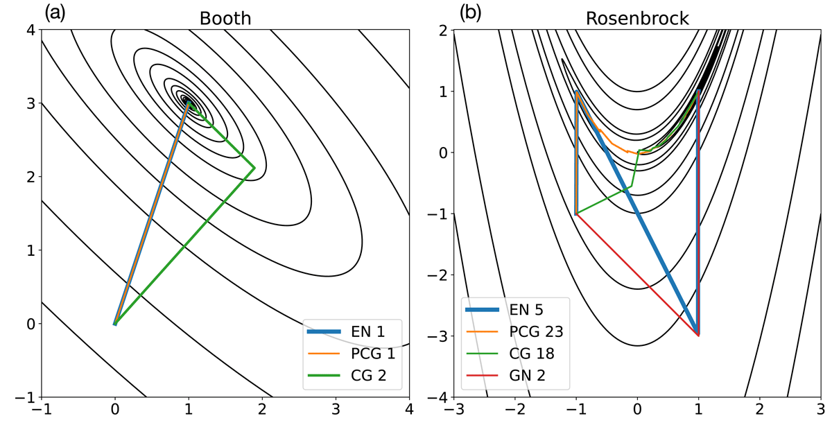
Figure 1
Minimisation of the (a) Booth and (b) Rosenbrock functions with the exact Newton (EN, blue), conjugate gradient (CG, green), preconditioned CG (PCG, orange) and Gauss–Newton (GN, red). Black contours are drawn in logarithmic intervals.
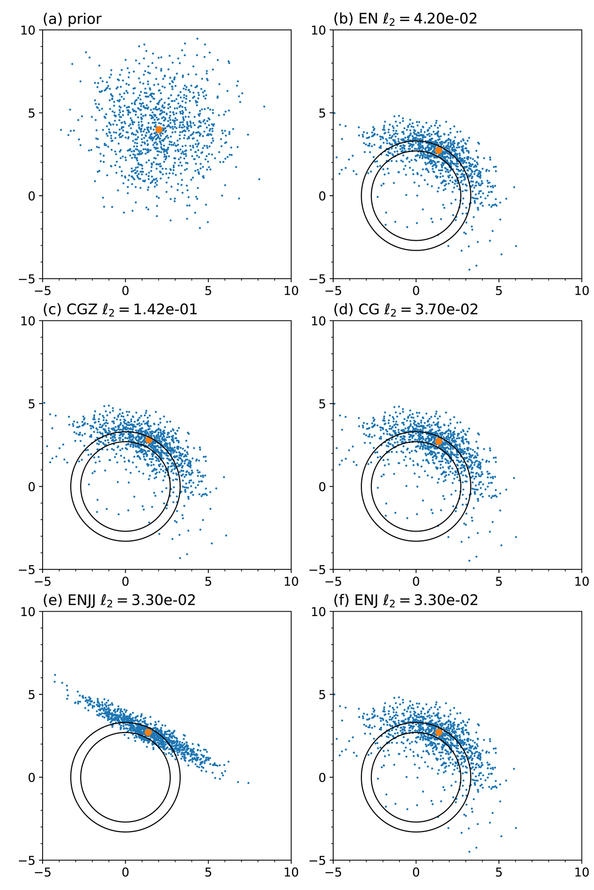
Figure 2
Distributions of (a) prior and posterior ensembles with the (b) exact Newton (EN), (c) conjugate gradient with updated Z (CGZ), (d) conjugate gradient with fixed Z (CG), (e) EN with the linearised observation operator applied during optimisation and the ensemble update (ENJJ) and (f) EN with the observation operator linearised during optimisation and approximated by ensemble on the ensemble update (ENJ), for the single wind speed assimilation. The orange dots represent the control forecast in (a) and the control analysis in (b)–(d). The wind speed observation is marked with the circles of radius 3.0 ± 0.3, ms–1. The title of each panel shows the optimisation method and ℓ2 analysis error.
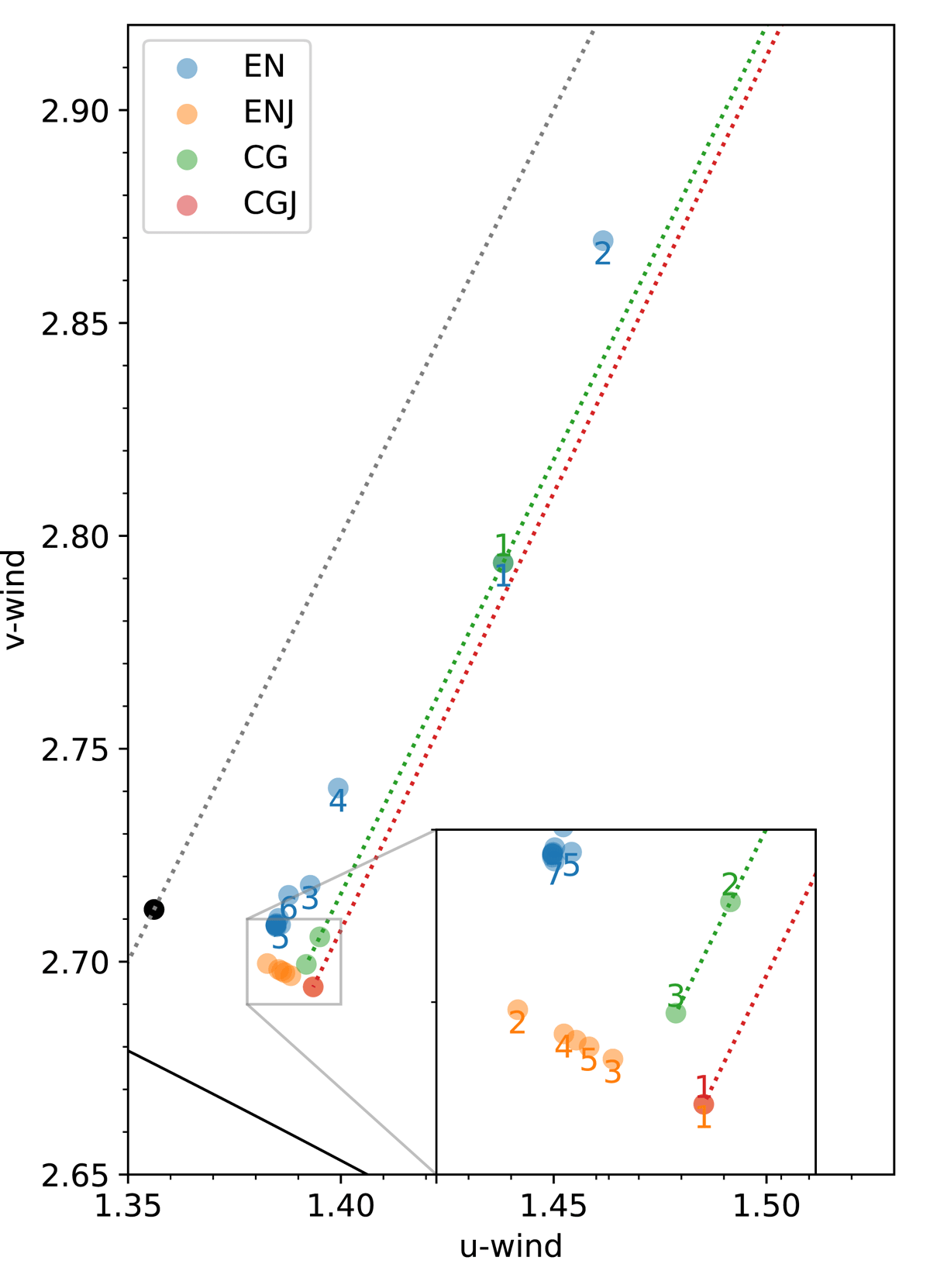
Figure 3
Intermediate values of the zonal and meridional winds (ms–1) during optimisation for the single wind speed assimilation. The number below and above a dot represents the number of iterations for the exact Newton (EN, blue)/EN with the analytical Jacobian (ENJ, orange) and conjugate gradient (CG, green)/CG with the analytical Jacobian (CGJ, red), respectively. The curve at the bottom left corner shows a part of circle |u| = 3.0 ms–1. The dotted grey line represents the steepest descent direction connecting the first guess and the origin. The green and red dotted lines represent the descent directions for CG and CGJ, respectively, connecting the first guess and the analysis. The black dot represents the analytical solution.
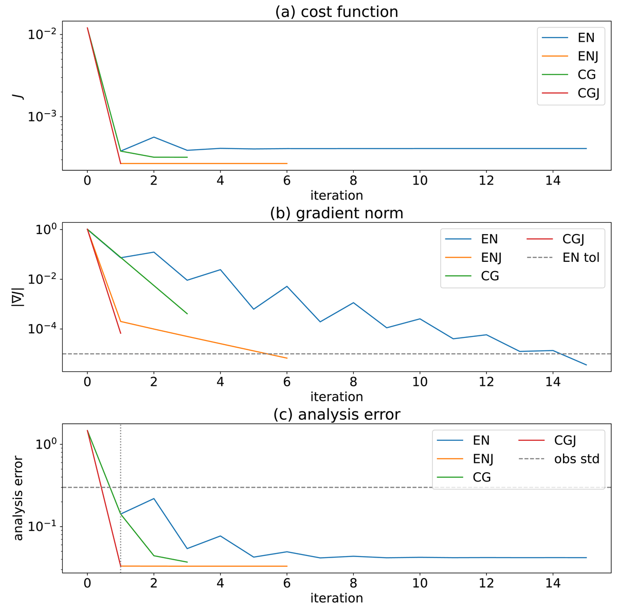
Figure 4
Changes in the (a) cost function, (b) gradient norm and (c) analysis error during iterative optimisation for the single wind speed assimilation with the exact Newton (EN, blue), EN with the Jacobian (ENJ, orange), conjugate gradient (CG, green), and CG with the Jacobian (CGJ, red). The tolerance of the EN gradient norm (10–5) is represented as a broken grey line in (b). The gradient norm of CG/CGJ is plotted with a scaling of . The observation standard deviation and the first iteration are marked by broken horizontal and dotted vertical lines, respectively, in (c).
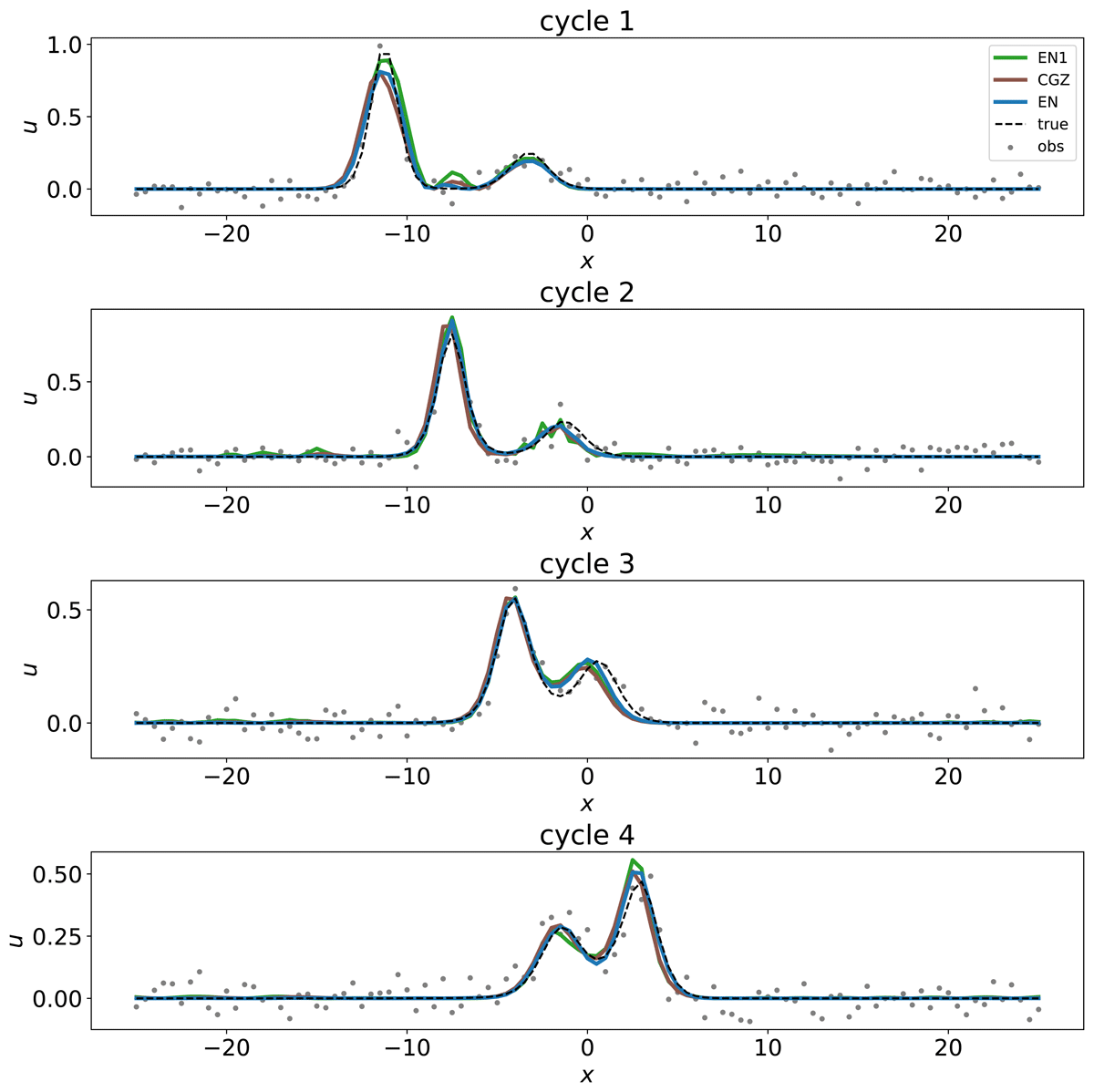
Figure 5
Analysis using the exact Newton (EN, blue), conjugate gradient with updated Z (CGZ, brown) and EN terminated at the first iteration (EN1, green) for the first four cycles with the Korteweg–de Vries–Burgers model. The black broken curve and grey dots represent the true run and its observations, respectively.
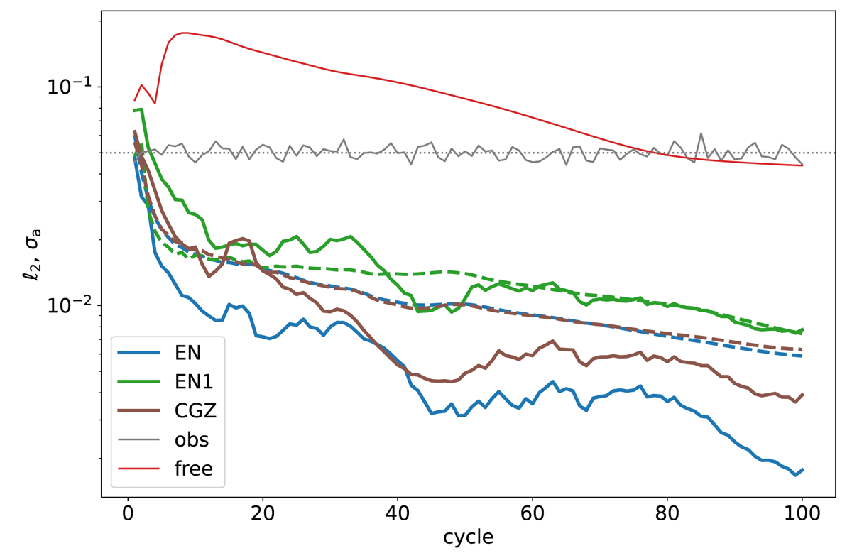
Figure 6
Analysis RMSE (solid) against the true run and analysis ensemble spread (dashed) for the data assimilation experiments over 100 cycles with the Korteweg–de Vries–Burgers model using the exact Newton (EN, blue), conjugate gradient with updated Z (CGZ, brown), and EN terminated at the first iteration (EN1, green). The grey and red curves show the prescribed (dotted) and actual (solid) observation error, and RMSE for the free run without data assimilation, respectively.
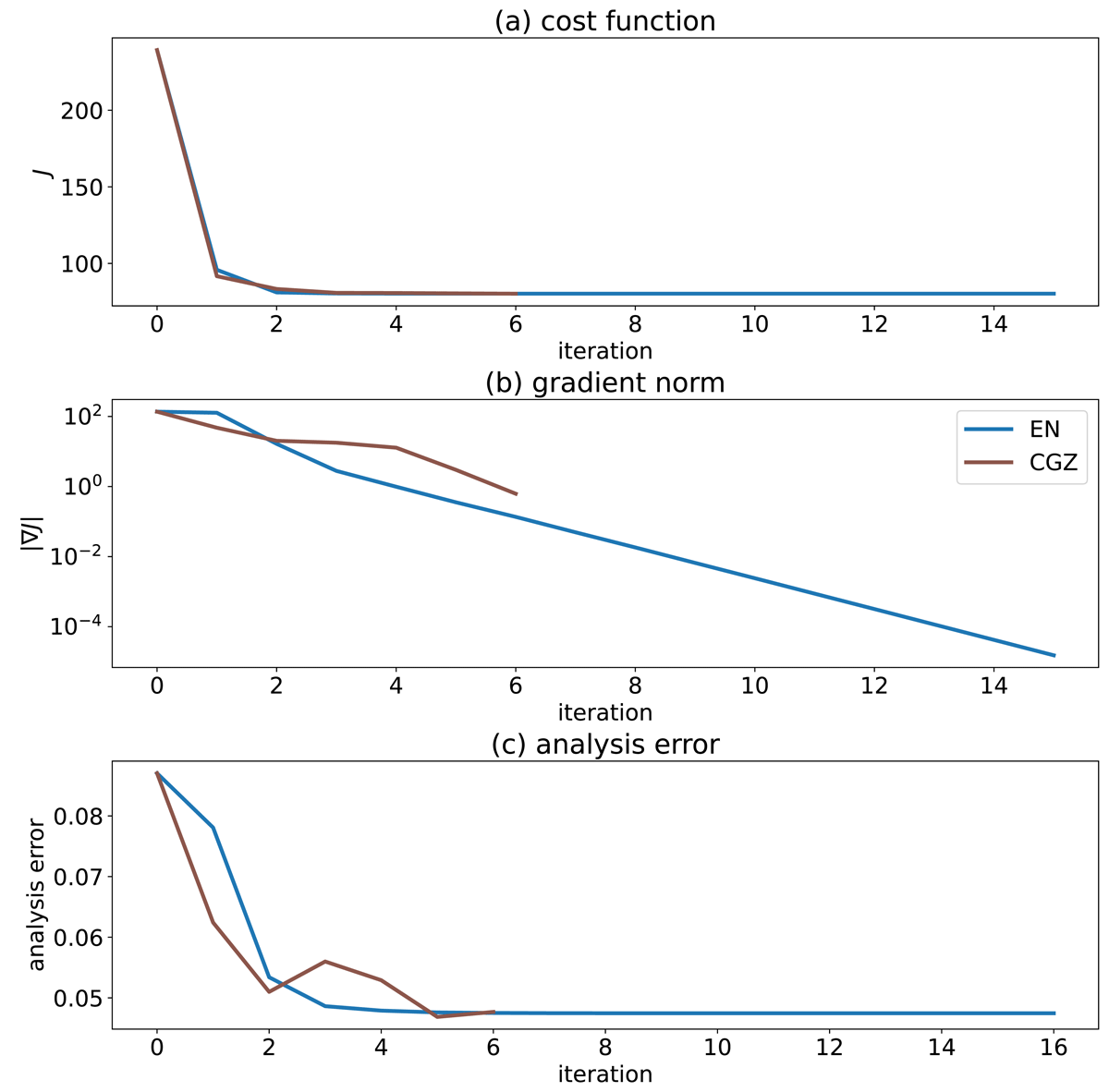
Figure 7
As in Figure 4 but for the first analysis cycle with the Korteweg–de Vries–Burgers model using the exact Newton (EN, blue), conjugate gradient with updated Z (CGZ, brown). The gradient of CGZ is plotted with a scaling to match that of EN at the beginning of the iterations.
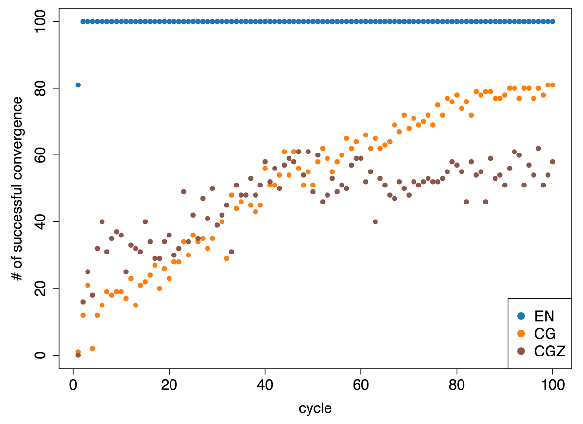
Figure 8
Number of successful convergence in data assimilation experiments with the exact Newton (EN, blue) and conjugate gradient with fixed and updated Z (CG, orange and CGZ, brown, respectively) using the Korteweg–de Vries–Burgers model.
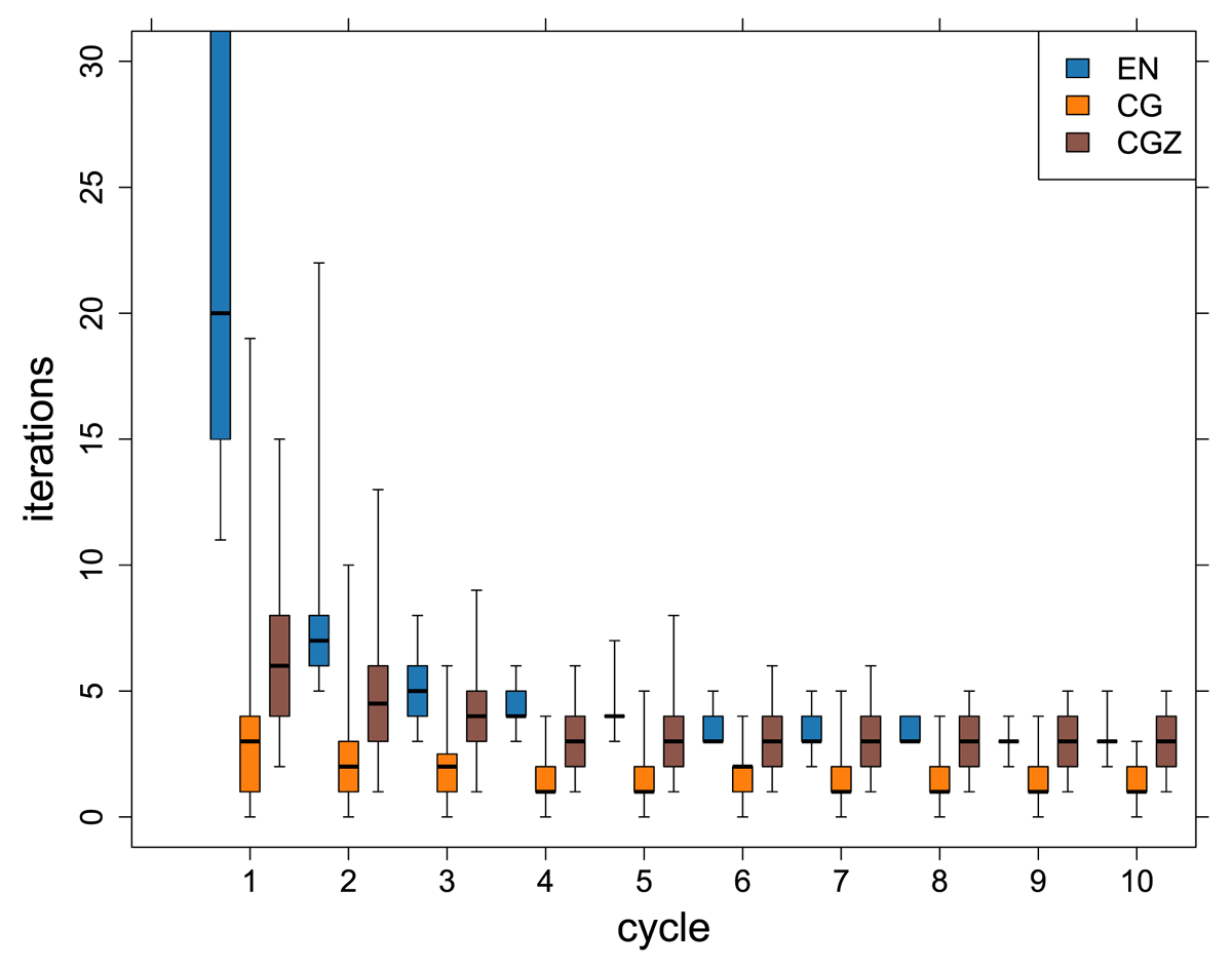
Figure 9
Number of iterations for the first 10 cycles in data assimilation experiments with the exact Newton, (EN, blue) and conjugate gradient with fixed and updated Z (CG, orange and CGZ, brown, respectively) using the Korteweg–de Vries–Burgers model. The thick lines represent the medians, the bottom and top of the box are first and third quadrants, and the minimum and maximum values are marked by whiskers.
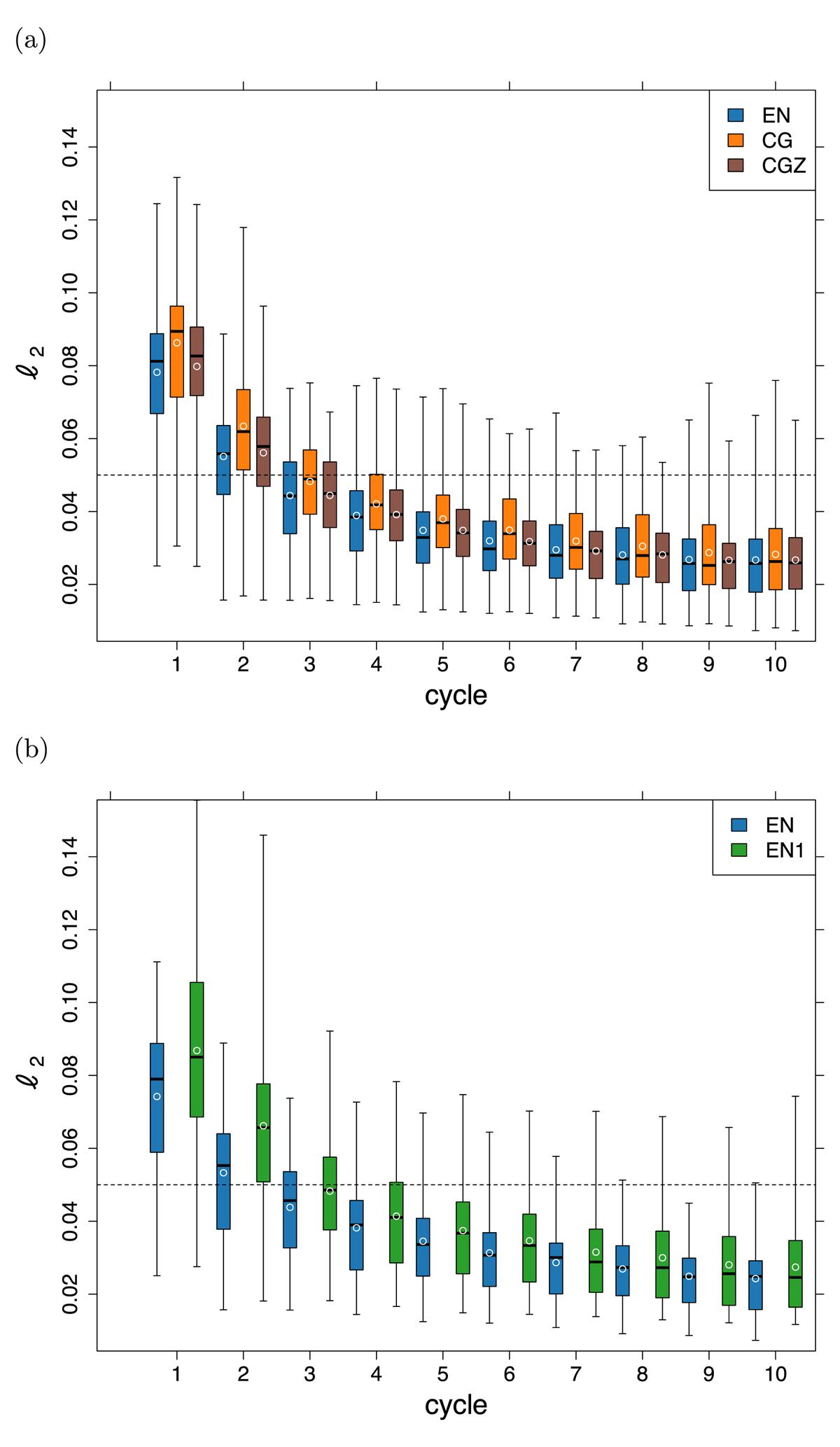
Figure 10
Two-norm error with the (a) exact Newton (EN, blue) and conjugate gradient with fixed and updated Z (CG, orange and CGZ, brown, respectively) (b) EN and EN terminated at the first iteration (EN1, green) with the Korteweg–de Vries–Burgers model for 81 and 42 successful tests of CG and EN1, respectively. The means for each cycle are represented by white circles.
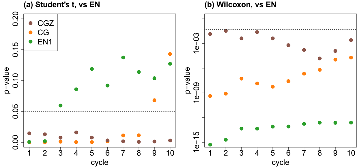
Figure 11
The p-values in paired Student’s t-tests (a) and those in Wilcoxon signed rank tests for (b) with the Korteweg–de Vries–Burgers model. The conjugate gradient with fixed (CG, orange) and updated Z (CGZ, brown), respectively, vs exact Newton (EN), and EN terminated at the first iteration (EN1, green) vs EN.