
1 Introduction
Optimisation of a cost function is a key component in variational data assimilation (VAR) and determines the analysis quality. For atmospheric applications, popular choices include the conjugate gradient (CG) method and quasi-Newton methods, such as the limited-memory Broyden–Fletcher–Goldfarb–Shanno (L-BFGS) method (Navon and Legler 1987). The CG method searches mutually conjugate directions, while quasi-Newton methods progressively approximate the Hessian from the initial guess, typically an identity matrix. A small footprint of several vectors is one of the benefits of these gradient-based optimisations for large-scale problems in VAR.
The control variable for optimisation may be transformed and alternatively be optimised in an ensemble space (Lorenc 2003). Due to the complexity of the forecast model, a typical ensemble size is O(10)–O(100), O(1000) at most. For such a problem size, the linear system can be solved, and a matrix can be inverted efficiently and accurately with a direct solver. The storage and computational load for the Hessian and its inverse are prohibitive in the physical space but tractable in an ensemble space. The Newton method exactly solves the quadratic approximation of the cost function and has quadratic convergence. The Newton method may or may not be used with a line search. In contrast, the CG and quasi-Newton methods with a line search (Nocedal and Wright 2006) inexactly solve the Newton equation and have linear and superlinear convergence, respectively.
The maximum likelihood ensemble filter (MLEF, Zupanski 2005) is a deterministic ensemble square-root filter that maximises the posterior probability distribution (maximum a posteriori estimation). The MLEF can be regarded as an ensemble VAR (Liu et al. 2008) as it can produce an analysis by minimising the cost function in the ensemble space using a nonlinear unconstrained optimisation method, such as CG or L-BFGS. The use of an ensemble eliminates the need for tangent linear and adjoint models and provides a flow-dependent forecast error covariance matrix. In addition, the Hessian can be calculated from an ensemble. In the MLEF, the Hessian is used for preconditioning by transforming the control variable to accelerate convergence. The MLEF can be formulated to accommodate non-differentiable observation operators (Zupanski et al. 2008) and non-Gaussian cost functions (Fletcher and Zupanski 2006).
The MLEF can improve an analysis by iteratively minimising the cost function and can effectively extract information from nonlinear observations. However, the minimisation with CG or quasi-Newton methods is often discontinued before reaching the minimum, and sometimes the analysis is not improved from the first iteration. This paper applies the Newton method to the MLEF and examines the analysis convergence and accuracy. The Newton equation is exactly solved without a line search at each iteration, hence called the exact Newton (EN) method. It should be noted that ‘exact’ does not refer to the exact solution of the line search subproblem. The Kalman gain calculation is equivalent to exactly solving the Newton equation (Zupanski 2005). The Gauss–Newton (GN) or Newton methods were chosen for the iterated Kalman smoother (Bell 1994) and for the iterative ensemble Kalman filters (Gu and Oliver 2007; Sakov et al. 2012). However, the advantages of the Newton method and its convergence properties are not necessarily obvious.
In this study, EN is compared against CG with Hessian preconditioning under the MLEF framework. Section 2 revisits optimisation with CG and EN with the Booth and Rosenbrock (1960) benchmark functions. Section 3 reviews the MLEF formulation and derives an alternative formulation using the EN method. Section 4 presents the assimilation of a single wind speed observation (Bowler et al. 2013) and cycled experiments with a Korteweg–de Vries–Burgers (KdVB) equation model (Zupanski 2005). Section 5 presents the summary and final remarks.
2 Optimisation of Benchmark Functions
This section applies the CG and EN methods to optimisation of two-dimensional Booth and Rosenbrock (1960) functions, which are expressed as a sum of squares of functions
The minimisation of the functions of this form is called linear or nonlinear least-square problems, depending on the linearity of residuals fi(x). The Booth function is a quadratic function with linear residuals, which is analogous to a cost function with a linear observation operator. Meanwhile, the Rosenbrock function is quartic function with a nonlinear residual, which is reminiscent of a quadratic observation operator.
The two functions are optimised with the CG method (Appendix A) with a line search (Appendix B), the preconditioned CG method (PCG), and the EN method (Navon and Legler 1987). The Rosenbrock function is also optimised by the Gauss–Newton method (GN). The quadratic approximation of a function f(x) is obtained by a truncated Taylor series
where d is a descent vector, and are the gradient vector and the Hessian at x, respectively. The minimum of (2) is achieved by solving the Newton equation
The GN method is often used to solve a nonlinear least-square problem. GN uses a Jacobian matrix
where f is called a residual vector, to approximate the gradient
and the Hessian
ignoring the contribution from the Hessian of the residual vector . The solution of the Newton equation becomes
The preconditioning can be done by a transform with a square root of the Hessian as
In PCG, the descent direction is updated by the same way as CG but the state vector x is preconditioned using the Hessian . Thus, the first descent direction of PCG becomes the Newton direction.
2.1 Booth function
The Booth function is defined by
in two dimensions. Unlike the sphere function (a circle in two dimensions) two variables are correlated, i.e. the off-diagonal elements of the Jacobian matrix are nonzero. The squashed shape and small gradients near the solution (1, 3) cause the minimisation with a simple optimisation method, such as the steepest descent method, challenging and demanding numerous iterations with a small step size. With f1(x, y) = x + 2y – 7 and f2(x, y) = 2x + y –5, a square root of the Hessian
yields x′ = x + 2y, y′= 2x + y; therefore, (9) is preconditioned to be
Minimisation is conducted with EN, CG, and PCG methods with the initial position at (0, 0). As expected, the EN and CG methods require only one and two steps to the solution, respectively (blue and green curves in Figure 1a). Here, the line search in CG is exact for the quadratic function. Preconditioning using the Hessian of (9) leads to the diversion of the descent direction of CG from the steepest to Newton directions and enables convergence in a single step (PCG, orange in Figure 1a), indicating that the Hessian preconditioning works effectively for quadratic cost functions.
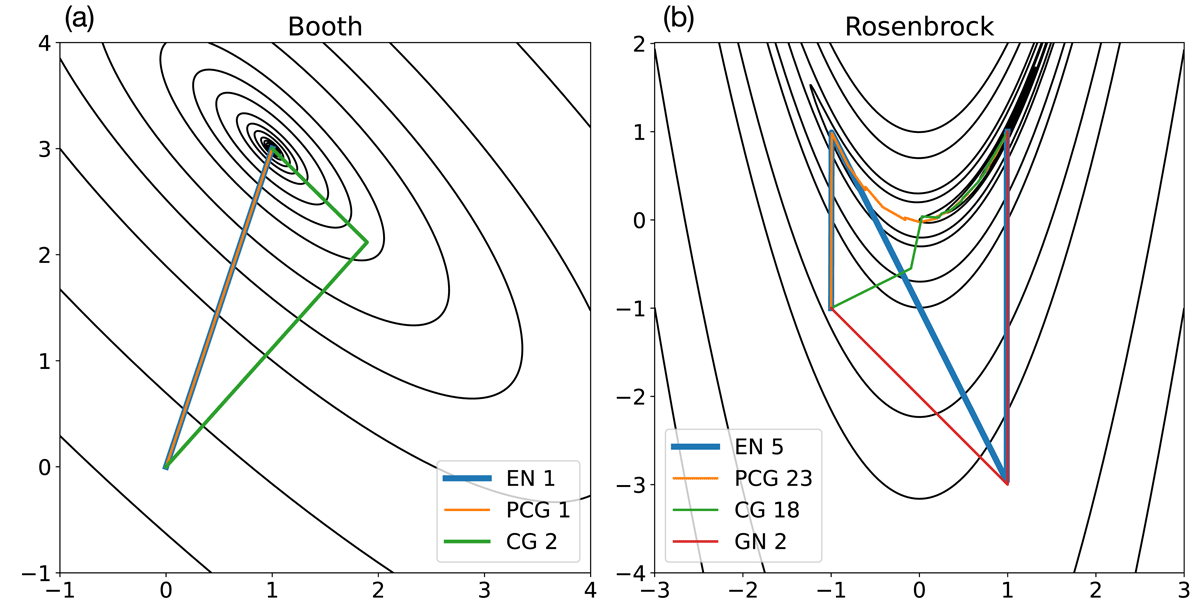
Figure 1
Minimisation of the (a) Booth and (b) Rosenbrock functions with the exact Newton (EN, blue), conjugate gradient (CG, green), preconditioned CG (PCG, orange) and Gauss–Newton (GN, red). Black contours are drawn in logarithmic intervals.
2.2 Rosenbrock function
The two-dimensional Rosenbrock function is defined by
with standard parameters. The optimisation is initiated at (–1, –1) with the control vector (x, y) for EN, CG and GN, and with (x′, y′) for PCG. The residual functions are defined as described in Appendix C. It should be noted that the behaviours of the optimisation schemes are not affected by the initial position except for x = 1 as discussed below. The gradient norm below 10–5 is used as a criterion for convergence. A banana-shaped valley hinders convergence and usually requires more iterations to reach the minimum at (1, 1).
CG (green in Figure 1b) starts with the steepest descent direction and falls into the ditch in two steps. The minimisation continues along the ravine before arriving at the minimiser in 18 steps. EN (blue) dives into the abyss in a single step but climbs the hill at the second step. The Rosenbrock function is minimised in a total of five steps, significantly fewer than CG. PCG (orange) shares the first descent direction with EN caused by the Hessian preconditioning. Unfortunately, PCG drops into the valley farther away from the goal at the first step and spends 23 iterations, with an increase of 5 steps from CG. GN (red), with the Hessian approximated by Jacobian matrix, converges in only two steps. The GN or EN methods with a line search (not shown) are conservative and guarantee a smaller cost than the initial value at the expense of slower convergence as CG and PCG.
The GN and EN tracks imply that an erroneous solution due to the increase of the cost can be obtained when the iterations are terminated at first and second steps, respectively. The descent vector of EN (and PCG) is not directed towards the minimiser, indicating adverse effect of the higher order derivatives. The Hessian approximated with the Jacobian matrix is no better than the full Hessian since it also leads to a state distant from the solution. However, it is an vantage point x = 1, where the Rosenbrock function (12) is a quadratic function f(y) = 100(y-1)2; therefore, it leads to the minimiser in the next step. The Jacobian-based Hessian that ignores second and higher derivatives is consistent with the quadratic assumption of the cost function. It should provide a good approximation of the full Hessian near the solution and reduces an error due to the inaccurate higher order derivatives away from the solution. Therefore, the Jacobian matrix can be beneficial when available. The EN and GN outperformance can be explained by obtaining the descent vector analytically in Appendix C.
3 Formulations
This section summarises the original MLEF formulation (Zupanski 2005; Zupanski et al. 2008) and describes our modifications.
Assuming the Gaussian distribution, the cost function may be written as
where x represents the state vector, i.e. the control variable of iterative minimisation, xf and y represents the first guess of the control forecast and observation, respectively; B and R are the background and observation error covariance matrix, respectively; and H is a nonlinear function that represents the observation operator. In ensemble-based data assimilation, the forecast error covariance matrix Pf approximates the background error covariance matrix. Each column of the square root of Pf is taken to be the deviation from the first guess xf for the corresponding ensemble forecast.
where k is the ensemble size,
and are the forecast and analysis perturbations, respectively. The departure of the state x from the control forecast xf is represented by a linear combination of ensemble perturbations with a weight w defined as
In terms of the ensemble weight w as the control variable, the cost function (13) may be written as
In this form, the background (first) term of the cost function (17) is quadratic in w and its Hessian is the identity matrix, but the observation (second) term is not quadratic unless the observation operator is linear.
In the following subsections the original and proposed methods are described. Because the original method does not specify which optimisation method to be used, CG is chosen in this study. The proposed method uses EN for optimisation.
3.1 Hessian preconditioning
The original MLEF employs the square root of the Hessian to precondition the forecast error covariance matrix in the following form
where and is the Hessian, and
is a normalised ensemble perturbation matrix in the observation space. When the Jacobian matrix is available, Z can be directly calculated by (19). With an ensemble, Z is approximated by the difference of the simulated observations between the perturbed and control states as
At the beginning of iterations, Z is calculated using x = xf and using x with (18) when it is updated.
In terms of the transformed control variable ζ, the cost function and gradient can be written as
and
respectively. Prior to the optimisation, the eigenvalue decomposition is used to compute the inverse of the Hessian and its square root, which are used consistently during iterations to evaluate the cost function (21) and its gradient (22).
After the minimisation, the ensemble update is performed with the optimised ensemble perturbation matrix in the observation space ,
The transposed square root of the inverse Hessian is calculated with the eigenvalue decomposition
In this study, PCG (simply denoted as CG hereafter) is used for optimisation with a line search (Appendix B.) It should be noted that ZT in (22) can be either fixed or updated during iterations. The CG using updated Z is similar to EN described in Subsection 3.2 in which Z is updated during iterations. The choice has a profound influence on optimisation hence the analysis, as will be shown in the data assimilation experiments (Section 4).
3.2 Exact Newton optimisation
The original solution method is modified to improve convergence and accuracy by using the Newton method. In addition, the proposed formulation avoids the square root matrices except for the ensemble update. The quadratic approximation of (17) is obtained by a truncated Taylor series
whose minimum is achieved by solving Newton equation
where the gradient vector and Hessian are
and
respectively, and
is an unnormalised ensemble perturbation matrix in the observation space. Here, Y is adopted instead of the normalised ensemble perturbation matrix in the observation space Z to avoid the inverse square root of the observation error covariance matrix. As for the normalised case, Y can be approximated by the difference
In (26), and d are called the steepest descent and Newton directions, respectively. These two directions coincide when the Hessian is an identity matrix, which is the case for the initial step for the CG and quasi-Newton methods with the Hessian preconditioning. To solve (26), the Hessian is not explicitly inverted but implicitly used in the linear system solution for the Newton equation because the linear system solution is numerically more accurate and stable than the inverse. It should be noted that eigenvalue decomposition is not performed here because the inverse square root of Hessian is not required.
As with ensemble Kalman filters the Newton equation (26) is solved exactly for the linear observation operator. The quadratically approximated Newton equation (26) is solved iteratively for a nonlinear observation operator. The gradient vector (27) and Hessian (28) are updated during minimisation for the weight w with innovation y – H(x) and ensemble perturbation matrix in the observation space Y. The ensemble update is analogous to the original scheme (23) except for the use of the Hessian (28) with Y recomputed using the analysis xa in (30).
The method in this study differs from the original in the following aspects. First, instead of the CG or a quasi-Newton method with Hessian preconditioning, the Newton equation is solved exactly, avoiding re-evaluation of the cost function (21) in the iterative line search subproblem. Second, the Hessian is updated during iterations, and its inverse is not explicitly computed. Finally, the square root of inverse of the observation error covariance matrix is not used. The off-diagonal elements of R are assumed to be naught in this paper but are nonzero in general. The proposed method avoids a non-unique square root of R and its computational cost. The original and the proposed methods yield the identical analysis for the linear observation operator, but can behave differently for nonlinear observation operators or for R with non-zero off-diagonal elements, due to the different optimisation methods and to non-uniqueness of the square root, respectively.
4 Data Assimilation Experiments
The two optimisation methods (EN and CG) in MLEF are compared in idealised data assimilation experiments. Unlike those analytically given for the benchmark functions in Section 2, the cost, gradient and Hessian are typically approximated with ensemble members. First, the two methods are validated without a forecast model in the assimilation of a single wind speed observation with an ensemble normally distributed around a first guess. Cycled experiments are then conducted with the KdVB equation model.
4.1 Assimilation of a single wind speed observation
The transform between the wind vector u and its magnitude |u| and direction θ is nonlinear.
This is identical to a transform between Cartesian and polar coordinates for object tracking besides the definition of the direction. A Gaussian distribution in the magnitude–direction space can be distorted in a banana shape with a small magnitude error and a large angle error. The linear transformation not only underestimates the covariance but also yields a biased posterior mean (Julier and Uhlmann 2004).
An assimilation of a single wind speed observation tests this nonlinear observation operator (the inverse of (31)) (Lorenc 2003; Bowler et al. 2013). The test uses a forecast ensemble with a size of k = 1000 distributed with a standard deviation of σu = σv = σf = 2 ms–1 around the first guess at xf = (2, 4) ms–1 (Figure 2a) and a single wind speed observation of Vo = 3 ms–1 with an error standard deviation of σo = 0.3 ms–1. Using the linearised observation operator H = u/|u|, this problem has the analytical solution of the form
where
and . For the above settings, the analytical solution is Va = 3.03 ms–1 and xa = (1.36, 2.71) ms–1. Iterations are terminated if the maximum number of steps (100) is reached or the gradient norm satisfies a criterion. EN is deemed converged when the gradient norm becomes smaller than 10–5. CG uses a smaller threshold of approximately 1.5 × 10⁻⁶ considering the transformation of the control vector (18). To determine the criterion for CG, that for EN is scaled with a factor that represents the Hessian preconditioning. With MLEF, the control forecast is used as the first guess and the anomalies from the control forecast are used as the square-root forecast error covariance matrix. This assumption leads to the ratio of the forecast to observation error covariance k times larger than . To be consistent with the specified background–observation error ratio, R is multiplied by k.
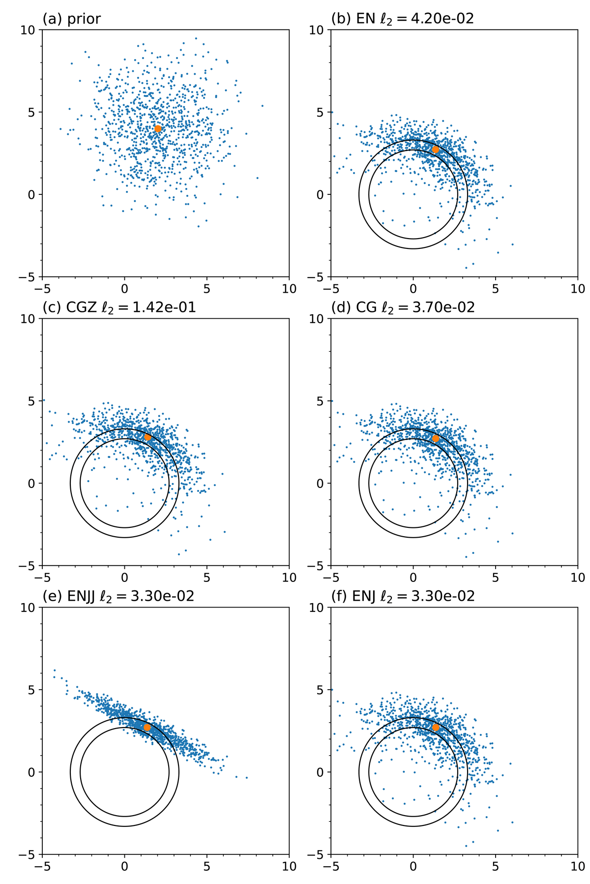
Figure 2
Distributions of (a) prior and posterior ensembles with the (b) exact Newton (EN), (c) conjugate gradient with updated Z (CGZ), (d) conjugate gradient with fixed Z (CG), (e) EN with the linearised observation operator applied during optimisation and the ensemble update (ENJJ) and (f) EN with the observation operator linearised during optimisation and approximated by ensemble on the ensemble update (ENJ), for the single wind speed assimilation. The orange dots represent the control forecast in (a) and the control analysis in (b)–(d). The wind speed observation is marked with the circles of radius 3.0 ± 0.3, ms–1. The title of each panel shows the optimisation method and ℓ2 analysis error.
4.1.1 Comparison between optimisation methods
EN and CG are compared in wind speed assimilation experiments. Figure 2 shows the prior and posterior distributions. As discussed in Section 3.1, the ensemble perturbation matrix in the observation space Z may be fixed (CG) or updated (CGZ) during iterations. The analysis (orange dot) falls within the observation standard deviation marked with double circles. The posterior ensembles (blue dots, in Figure 2b, c, d, f) look almost identical but differences exist in the ℓ2-norm error and convergence. EN converges in 15 steps while CGZ fails to converge due to the failure in the line search at step 1 (Figure 2b, c, respectively.) It turned out that the fixed Z acts as a remedy for the stagnation. CG can improve the solution further and converge in three steps (Figure 2d). The CG analysis error at the third step is reduced by approximately an order of magnitude from that of CGZ at the first step and comparable to that of EN at 15th step.
The reason why the remedy works can be explained as follows. A descent direction towards the origin leads to the solution (cf. H = u/|u|) because the observation Vo is any point on a circle of 3 ms–1. Therefore, the steepest direction should be selected at each iterative step. CGZ fails because g1 ≠ g0 for the updated Z to yield β1 ≠ 0 (38 in Appendix A), i.e. the contribution from the initial descent direction d0 = –g0, where the subscript denotes the counter of iterations and g is the gradient, remains and the descent direction is not the steepest descent direction at the first step. The cost function for the first step J(w1) is monotonically increasing and the line search fails to terminate the optimisation. CG descends along the steepest direction because thus βk = 0 (Appendix A).
4.1.2 Approximated and analyitical Jacobian matrices
CG with the Jacobian (CGJ) and EN with the Jacobian (ENJ) that use the analytical form H = u/|u| in (19) and (29), respectively, are compared against CG and EN to examine the influence of the finite-difference approximation of the Jacobian of the observation operator. The optimisation history in the zonal and meridional winds (Figure 3) shows that EN becomes closer and farther alternatively, corresponding to the cost oscillation (blue curve in Figure 4a). In addition, EN slightly staggers perpendicular to the descent directions, probably due to the error introduced by ensemble approximation of the gradient and Hessian, i.e. the Newton direction is not always towards the solution. CG with the fixed Z steadily approaches the solution in the Newton direction that is shared by the first step of EN and attains the minimiser in five steps. The first steps of CG and EN are identical due to CG’s step size of 1. ENJ jumps to a point very close but not identical to that of CGJ in a single step with an ℓ2 analysis error of 3.31 × 10⁻²; however, it moves along the circle for another five steps until the convergence criterion in the gradient norm is satisfied.
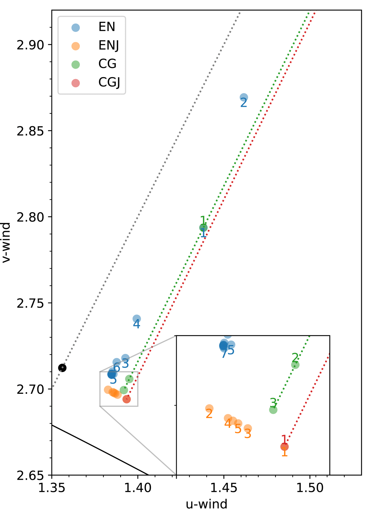
Figure 3
Intermediate values of the zonal and meridional winds (ms–1) during optimisation for the single wind speed assimilation. The number below and above a dot represents the number of iterations for the exact Newton (EN, blue)/EN with the analytical Jacobian (ENJ, orange) and conjugate gradient (CG, green)/CG with the analytical Jacobian (CGJ, red), respectively. The curve at the bottom left corner shows a part of circle |u| = 3.0 ms–1. The dotted grey line represents the steepest descent direction connecting the first guess and the origin. The green and red dotted lines represent the descent directions for CG and CGJ, respectively, connecting the first guess and the analysis. The black dot represents the analytical solution.
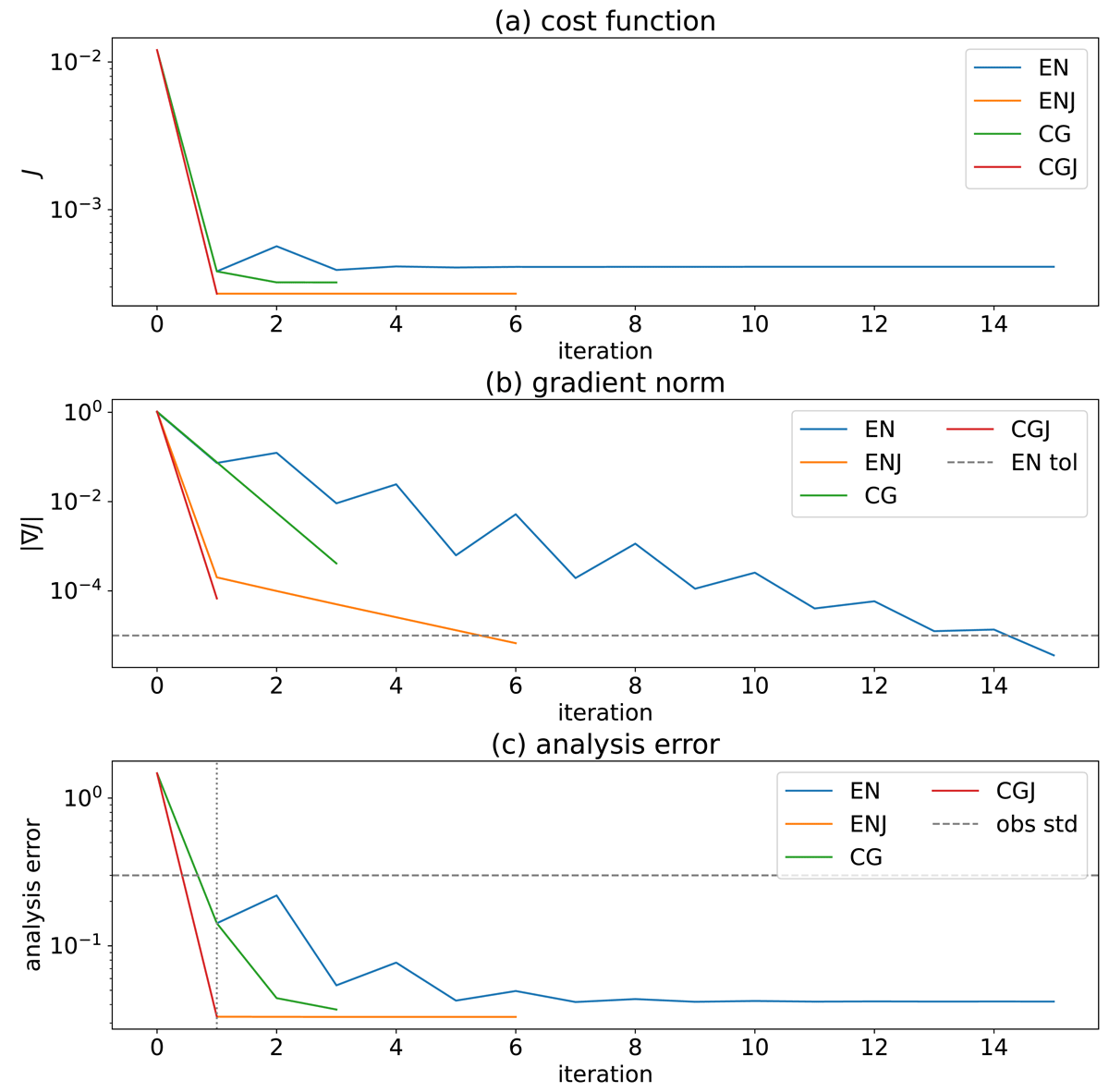
Figure 4
Changes in the (a) cost function, (b) gradient norm and (c) analysis error during iterative optimisation for the single wind speed assimilation with the exact Newton (EN, blue), EN with the Jacobian (ENJ, orange), conjugate gradient (CG, green), and CG with the Jacobian (CGJ, red). The tolerance of the EN gradient norm (10–5) is represented as a broken grey line in (b). The gradient norm of CG/CGJ is plotted with a scaling of . The observation standard deviation and the first iteration are marked by broken horizontal and dotted vertical lines, respectively, in (c).
The above result shows that the gradient and Hessian calculated from the ensemble can be inaccurate, unlike optimisation for the benchmark functions. CG is less sensitive to the approximation because the Hessian and the perturbation matrix Z are fixed before iterations. When available, it is better to use the analytical Jacobian to avoid the finite-difference error. However, ensemble members are aligned around the tangent to a circle at the analysis (ENJJ, Figure 2e) when the ensemble is updated with the ensemble perturbation matrix in the observation space (29) computed with the Jacobian of the observation operator. Therefore, the finite-difference approximation of the ensemble perturbation matrix in the observation space (30) is preferred for the ensemble update (ENJ, Figure 2f).
Figure 4 compares the cost functions, gradient norm and analysis error during iterations for the four optimisation methods. EN (blue) requires the largest number of iterations (15 steps) to satisfy the stopping criterion; however, the gradient norm decreases geometrically with diminishing oscillations and the changes of cost function are small from the third iteration. CG (green) is terminated in three steps but achieve the comparable error as the converged EN solution when Z is fixed otherwise CGZ stagnates at the first step. Using of the analytical Jacobian helps in achieving faster convergence (ENJ, orange; CGJ, red). The analysis error goes below the observation standard deviation and CGJ converges at the first iteration. Unlike EN, the cost function and gradient no longer oscillate with ENJ.
The single wind speed assimilation is a challenging problem for ensemble methods. The gradient and the Hessian matrix are inaccurate even with a large ensemble size of 1000 members. The observation operator is nonlinear and the cost function is not quadratic. Moreover, the cost function in the magnitude–direction space is quadratic, and the minimiser can easily be found by consistently proceeding towards the steepest descent direction. The quadratic nature of the problem can explain the effectiveness of the analytically obtained Jacobian and the fixed Z for CG.
4.2 Cycled experiments
This subsection validates EN against CG with a model of the Korteweg–de Vries–Burgers (KdVB) equation
where u is the model state, t and x are the time and space dimension, respectively, and ν is a diffusion coefficient. The inviscid case, where ν = 0 in (32), is called the Korteweg–de Vries (KdV) equation. The KdVB model is discretised in space and time with the centred finite-difference method and the fourth-order Runge–Kutta method, respectively (Marchant and Smyth 2002). The model configuration follows that of Zupanski (2005). There are grid points n = 101 with a spacing of Δx = 0.5. A time step of Δt = 0.01 and a diffusion coefficient ν = 0.07 is used for the control run. In this study, the model domain is chosen to be –25≤ x ≤ 25.
The initial state of the true run is taken from a two-soliton solution of the KdV equation. The two-soliton solution can be written as a sum of two single solitons for the regular (sech) and irregular (csch) solutions (Yoneyama 1984).
where
and β1,2 are Bäcklund parameters. The two-soliton solution (33) can then be rewritten with cosh as
The true run, from which observations are generated, and the control run, to which observations are assimilated, are integrated from the two-soliton solutions with β1 = 0.5 and β2 = 1.0 at t = –5 and with β1 = 0.4 and β2 = 0.9 at t = –6, respectively. The ensemble members of size k = 10 are generated as follows. The unperturbed run uses the same Bäcklund parameters as the control run but integrated from t = –7. For the perturbed runs, the Bäcklund parameters and initial time are perturbed with a standard deviation of (10% of β1 and β2) and σt = 2, respectively. The ensemble is integrated for 400 steps. The unperturbed run is subtracted from the perturbed runs to generate the initial perturbations and discarded. The perturbations are added to the control run to form the ensemble members. The Monte Carlo method is used to estimate the initial forecast error covariance, i.e. initial perturbations are scaled by . The scaling is not used during the cycle following the philosophy behind MLEF (Zupanski 2005) that error covariance is propagated by the model in a similar manner to the Kalman filter. An analysis is conducted every 200 model time steps. An observation is generated at every grid point by adding Gaussian noise of an amplitude 0.05 to the true run using a quadratic observation operator (H(u) = u2). Each experiment performs 100 analyses from t = –6.
4.2.1 Comparison for a particular realisation
The KdVB model is used to compare EN and CG in cycled data assimilation experiments with the same initial ensemble and observations. Deterministic (EN1) and iterative (EN) solutions are examined for optimisation effectiveness. Because the forecast is unstable for CG when the ensemble perturbation matrix in the observation space Z is fixed (CG), Z is updated during the analysis (CGZ).
Figure 5 shows the analyses for the first four cycles. EN (blue) is the smoothest solution with two peaks after cycle 2, and quickly converges to the true run (broken black). EN1 has short-scale noise that is most noticeable at cycle 2. All methods achieve an error below the observational error (grey) in several cycles, showing the effectiveness of data assimilation over the free run, in which error grows until about 10 cycles due to nonlinearity of the model (Figure 6). The final error for EN (blue) is almost an order of magnitude smaller than that for EN1 (green). In the middle of the cycles, CGZ reduces error significantly and is almost as good as EN, although the analysis error is saturated in all experiments, and the error of the free run even diminishes due to diffusion. Therefore, the several cycles from the beginning, where the error reduction is largest, are examined.
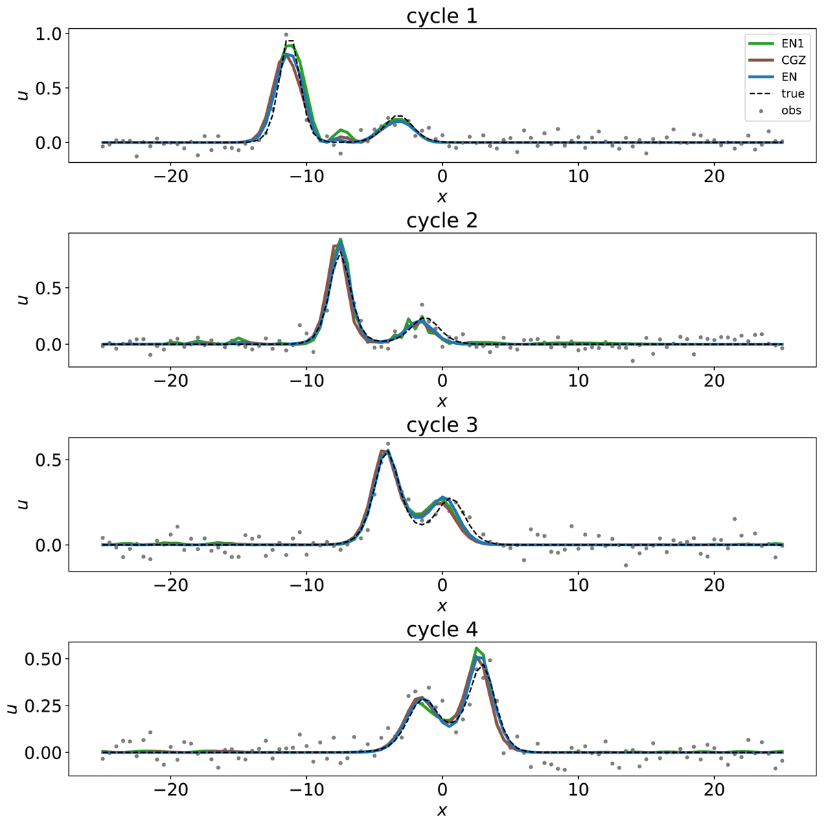
Figure 5
Analysis using the exact Newton (EN, blue), conjugate gradient with updated Z (CGZ, brown) and EN terminated at the first iteration (EN1, green) for the first four cycles with the Korteweg–de Vries–Burgers model. The black broken curve and grey dots represent the true run and its observations, respectively.
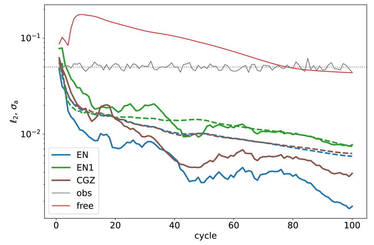
Figure 6
Analysis RMSE (solid) against the true run and analysis ensemble spread (dashed) for the data assimilation experiments over 100 cycles with the Korteweg–de Vries–Burgers model using the exact Newton (EN, blue), conjugate gradient with updated Z (CGZ, brown), and EN terminated at the first iteration (EN1, green). The grey and red curves show the prescribed (dotted) and actual (solid) observation error, and RMSE for the free run without data assimilation, respectively.
The iterative optimisations with EN and CGZ are compared for the first cycle in Figure 7. EN (blue) converges in 15 steps. After cycle 3, no further significant reduction is observed in the cost function and analysis error even though the gradient norm does not meet the stopping criterion. The cost function and gradient norm are reduced, but the analysis is slightly increased, implying the distance from the solution. CGZ (brown) benefits from the updated Z and achieves an analysis error as small as that of EN. The iteration is terminated before the gradient norm meets the criterion (10–5). The results are in contrast with the wind speed experiments, in which CG is optimised because the descent is guaranteed in the steepest descent direction computed for the first guess.
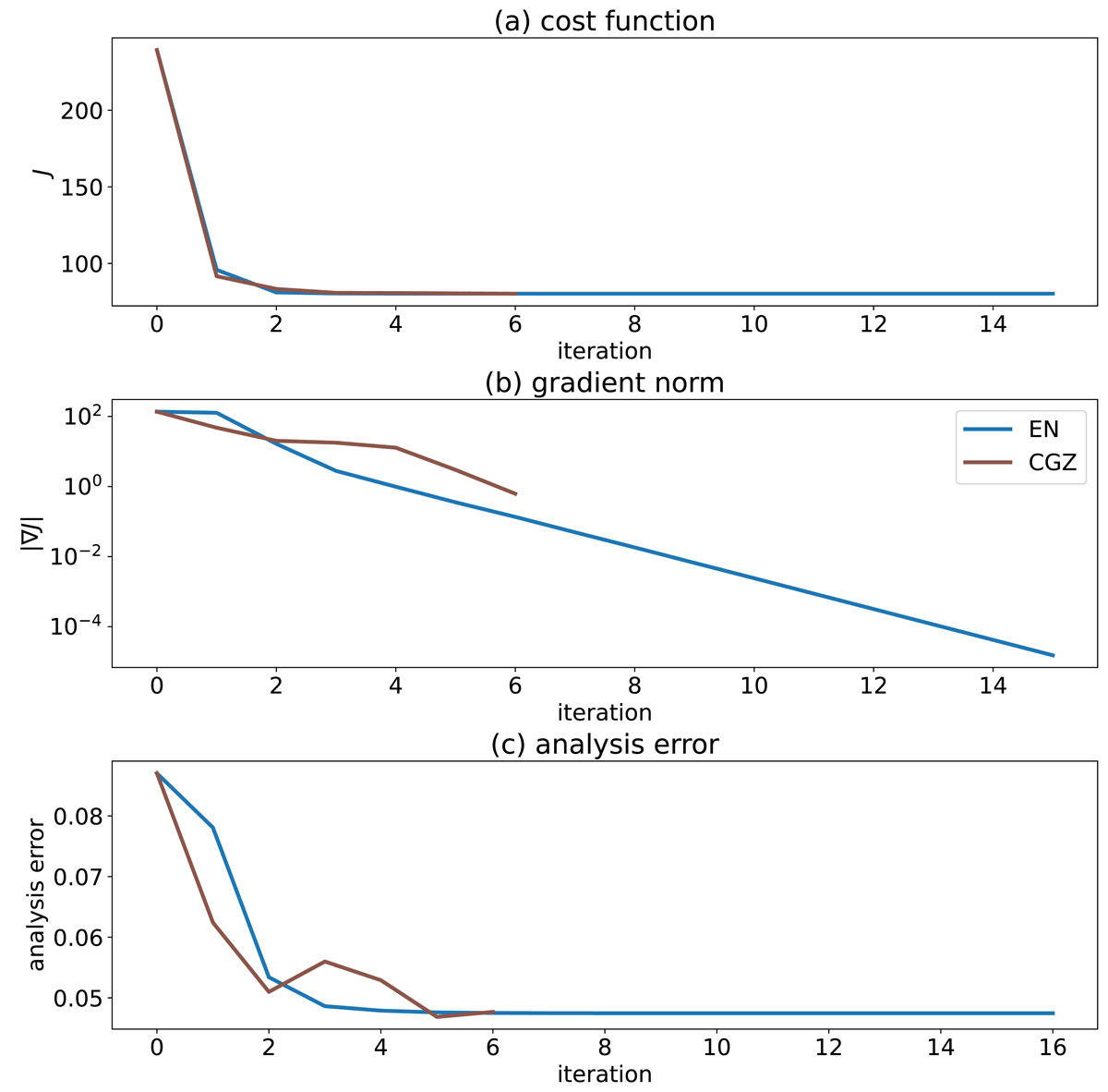
Figure 7
As in Figure 4 but for the first analysis cycle with the Korteweg–de Vries–Burgers model using the exact Newton (EN, blue), conjugate gradient with updated Z (CGZ, brown). The gradient of CGZ is plotted with a scaling to match that of EN at the beginning of the iterations.
4.2.2 Repeated tests
It turns out that the KdVB model may be unstable for a combination of certain initial ensemble and observations. In fact CG with the fixed Z failed for the ensemble and observations used in the Section 4.2.1. The stability of the analysis–forecast cycle with the MLEF and KdVB model are examined in a test repeated for 100 times. Each test uses a different realisation of an initial ensemble and observations. The numbers of successful tests are 100, 100, 81, and 42 for EN, CGZ, CG, and EN1, respectively.
Figure 8 compares the number of successful convergence for each cycle. EN (blue) always converges within 100 iterations except for the first cycle, where convergence is achieved in 81 tests. CG and CGZ never converges for the first cycle and convergence is achieved in equal to or less than 40 and 21 tests, respectively, for the first ten cycles. The number of successful convergence increases gradually with cycles with a median and maximum of 58 and 81 for CGZ and 51 and 62 for CG, respectively.
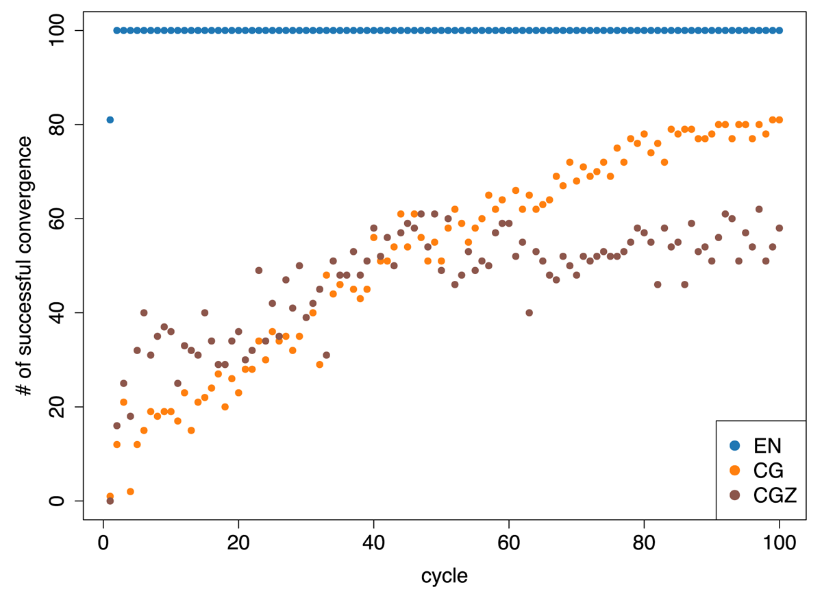
Figure 8
Number of successful convergence in data assimilation experiments with the exact Newton (EN, blue) and conjugate gradient with fixed and updated Z (CG, orange and CGZ, brown, respectively) using the Korteweg–de Vries–Burgers model.
EN consumes a greater number of iterations in the first five cycles than CG or CGZ (Figure 9). It should be noted that the boxes and whiskers include cases without convergence. The smaller numbers of iterations for CG or CGZ do not indicate faster convergence but immature termination and inability to continue minimisation. The medians of the number of iterations for EN are comparable to that for CGZ after cycle 6 and its variance is smaller. It should be noted that EN always converges after the first cycle and CG or CGZ does not in the majority of tests.
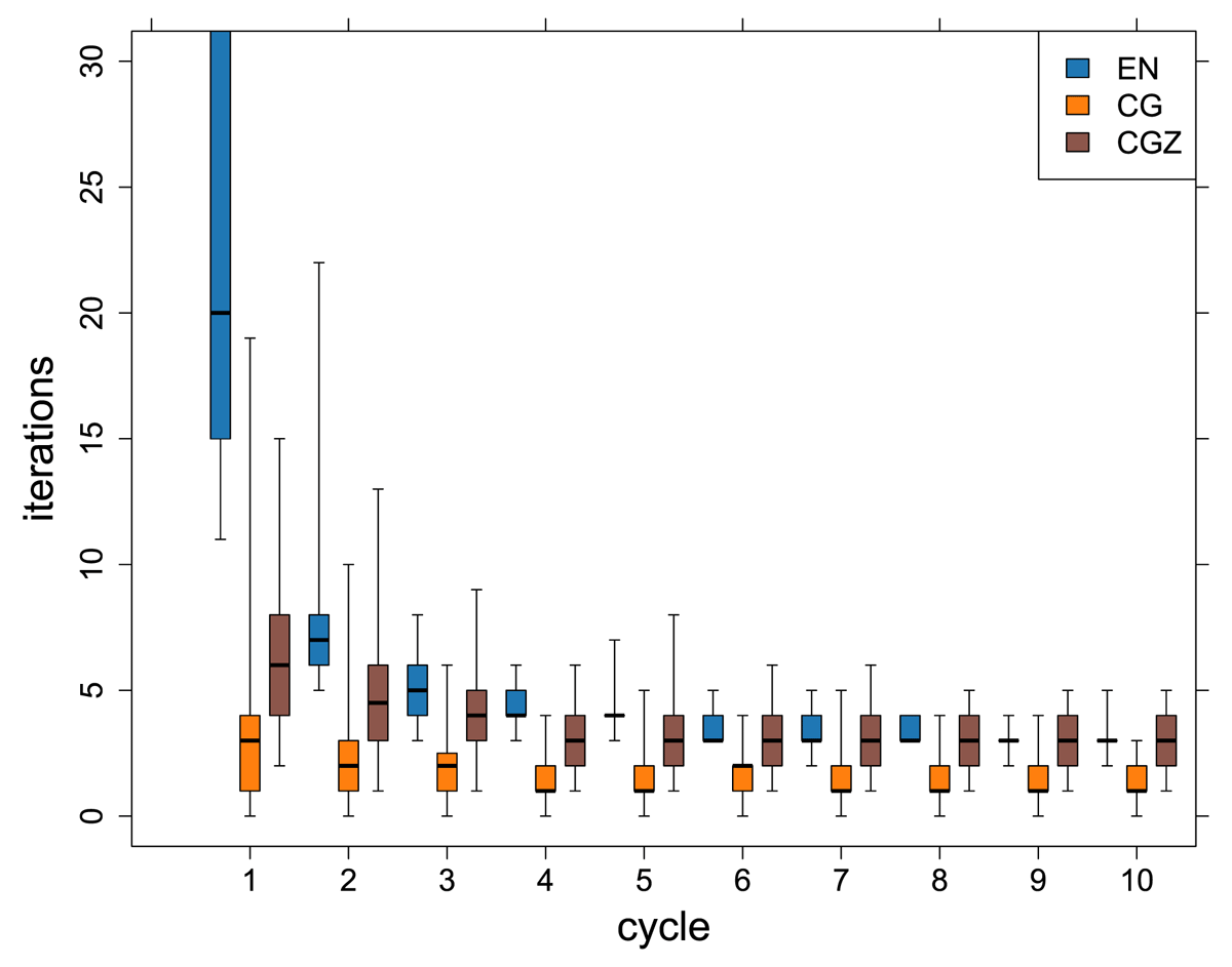
Figure 9
Number of iterations for the first 10 cycles in data assimilation experiments with the exact Newton, (EN, blue) and conjugate gradient with fixed and updated Z (CG, orange and CGZ, brown, respectively) using the Korteweg–de Vries–Burgers model. The thick lines represent the medians, the bottom and top of the box are first and third quadrants, and the minimum and maximum values are marked by whiskers.
The analysis error is compared in Figure 10. Figure 10a and b are plotted for 81 cases of EN, CG, CGZ and 42 cases of EN and EN1, respectively. Compared with CG, an error is indeed more effectively reduced with EN or CGZ especially in earlier cycles (Figure 10a). EN1 is inferior to EN statistically (the median, mean, minimum, maximum, first and third quantiles), indicating the optimisation effectiveness.
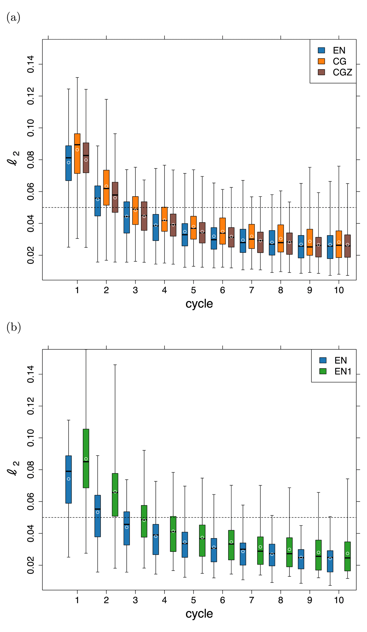
Figure 10
Two-norm error with the (a) exact Newton (EN, blue) and conjugate gradient with fixed and updated Z (CG, orange and CGZ, brown, respectively) (b) EN and EN terminated at the first iteration (EN1, green) with the Korteweg–de Vries–Burgers model for 81 and 42 successful tests of CG and EN1, respectively. The means for each cycle are represented by white circles.
To determine the statistical differences, paired Student’s t-tests and Wilcoxon rank sum tests are conducted (Figure 11) with a confidence level of 0.95. The null hypothesis is that the difference is insignificant. The alternative hypothesis is that the analysis error of CG, CGZ, or EN1 is greater than that of EN. In the Wilcoxon rank sum tests the ranks of the failed tests are set to the last place, i.e., 82th and 43th for CG and EN1, respectively. EN is significantly more accurate than CG up to the the first eight cycles in Student’s t tests and throughout the first ten cycles in the Wilcoxon rank sum tests. The advantage of EN over CGZ is clear both in Student’s t and the Wilcoxon rank sum tests. EN is significantly more accurate than EN1 only for the first two cycles in Student’s t-tests, but at all cycles in the Wilcoxon rank sum tests.
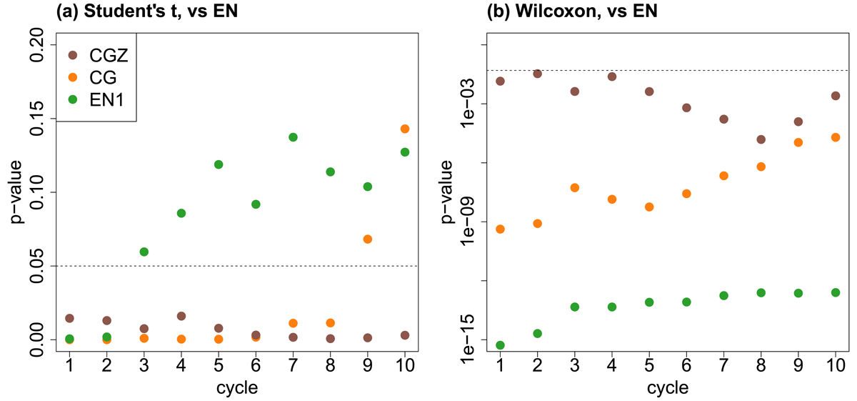
Figure 11
The p-values in paired Student’s t-tests (a) and those in Wilcoxon signed rank tests for (b) with the Korteweg–de Vries–Burgers model. The conjugate gradient with fixed (CG, orange) and updated Z (CGZ, brown), respectively, vs exact Newton (EN), and EN terminated at the first iteration (EN1, green) vs EN.
5 Summary and Discussion
A simplified variant of the MLEF has been proposed in which the cost function is minimised by exactly solving the Newton equation (EN) as an alternative to the original formulation of Zupanski (2005) using the Hessian for preconditioning and optimisation with a line search.
First, EN and CG methods are tested against two benchmark functions. The Hessian preconditioning effectively works for the Booth function, and both preconditioned CG and EN converge in a single step. This is not the case for the Rosenbrock function, but EN and GN converge fast, as discussed in Appendix C.
Then the modified MLEF has been validated with a single wind speed assimilation test and cycled experiments with a quadratic observation operator. The solutions with CG and EN for the wind speed assimilation are similar due to the comparable error. With CG, the normalised ensemble perturbation matrix in the observation space (Z) used to calculate the gradient must be fixed; otherwise, the optimisation cannot proceed beyond the first step and the analysis remains suboptimal. The gradient norm of EN reduces geometrically; however, it increases and decreases alternatively and the convergence is slower than that of CG with fixed Z. The number of iterations significantly reduced with analytical Jacobian is used, indicating influence from the error in the gradient and Hessian approximated by ensemble.
In the cycled experiments with the KdVB model, EN more effectively and efficiently minimises the cost than CG and yields outstanding stability. When the number of iterations is limited to 1, the analysis is degraded, and the forecast becomes unstable. The results of repeated tests indicate a statistically significant difference. The updates of Z are beneficial in CG, for the stability and accuracy of CG with the updated Z and EN are comparable for cycled experiments with the KdVB model. The superiority of EN or CGZ to CG probably stems from the updated observation perturbation matrix in ensemble space at each iterative step. EN and CGZ can use a better gradient than CG and EN can also take advantage of the updated Hessian.
MLEF with EN adaptively iterates depending on the distance from the solution. The maximum number of iterations is set 100, in this study, but only several iterations are required, except for the first few cycles. A smaller limit may be used to reduce computational cost. Alternatively, the limit is left large enough to let EN deal with a cycle in which observations are farther from the first guess.
The results show that EN has an excellent convergence property and can iteratively minimise the cost to yield optimal analysis for nonlinear observations in simple assimilation experiments with MLEF. Moreover, MLEF with EN is successfully applied to an atmospheric general circulation model SPEEDY (Molteni 2003) and a nonhydrostatic regional atmospheric model NCEP RSM (Juang 2000). It should be noted that practical considerations, such as inflation and localisation of the forecast covariance, are required for such large-scale problems. EN effectively minimises the cost function although the convergence is not always attained as with the KdVB model. The results with these models will be reported in separate papers.
A Conjugate Gradient Method
This appendix briefly describes the CG method as implemented in scipy.optimize (Polak and Ribière 1969; Navon and Legler 1987).
The initial descent direction is set to the steepest descent direction.
where the subscript indicates the number of iteration (0 for the initial position) and is a derivative of a function f(x) with respect to the state x.
The state is updated with
where αk is a step size that minimises (Appendix B).
The descent direction is updated as
where
When and the steepest descent direction is chosen as a descent direction as for the first descent direction d0, i.e. CG is restarted.
B Line Search
The line search subproblem finds the step size α > 0 such that
is minimised for the fixed state x and the descent direction d (Moré and Thuente 1994; Nocedal and Wright 2006).
To avoid possibly expensive function evaluations, an inexact line search is conducted with a sufficient decrease condition (Armijo condition)
and a curvature condition (strong Wolfe condition)
where 0 < c1 < c2 < 1. The parameters c1 = 1× 10⁻⁴ and c2 = 0.4 are used in scipy.optimize.minimize (method=’CG’). The first guess of the step size is 1 at the beginning and at n-th (n > 1) descent direction, where and . Then, the applicable step size is searched iteratively by try-and-error with suitable interpolations.
C Fast Convergence of Newton and Gauss-Newton Methods
The gradient vector, Hessian, and its inverse of the Rosenbrock function (12), which are required to solve the Newton equation (3), are derived from (12) as follows
Then the descent vector for each step is
Away from y = x2, the descent vector is d ≈ (0, –y+x2) because |200(y–x2)| is large and yields y ≈ x2. For y ≈ x2, 200(y–x2) is negligible, and the descent vector becomes d≈ (1–x, 2x(1–x)) and x ≈ 1 in the next step. Starting from x0 = (–1, –1), i.e. |200(y–x2)| = 400, x1 ≈ (–1, 1), i.e. y ≈ x2, x2 ≈ (1, –3), where the subscript denotes the number of iterations. Two more steps are required to exactly arrive at x = 1 where d = (0, 1–y) that moves the state to the minimum.
GN requires a Jacobian matrix to approximate the Hessian. The vector of residual functions for the nonlinear least squares (1) for the Rosenbrock function (12) are
The Jacobian matrix is composed of derivatives of the residuals
The gradient can be expressed exactly with the residual functions and the Jacobian matrix as and the Hessian is approximated by ignoring the second and higher derivatives.
The gradient and Hessian inverse
are combined to obtain the descent vector
The decent vector (51) leads x to 1 for any initial x and y to 1 for any y if x = 1. Consequently, the Rosenbrock function is minimised in only two steps with GN.
Data Accessibility Statement
The source code is available from https://github.com/tenomoto/kdvb.
Acknowledgements
Scipy is used for the linear algebra and conjugate gradient method. The authors thank Prof. Milija Zupanski for helpful discussions.
Funding Information
This research was supported by JSPS KAKENHI 19H05605, 21K03662 and 22KJ1966.
Competing Interests
The authors have no competing interests to declare.
Author Contributions
Takeshi Enomoto developed the code, conducted all the experiments and wrote the main text. Saori Nakashita conducted preliminary experiments, suggested experimental designs and contributed the interpretation of the results.