
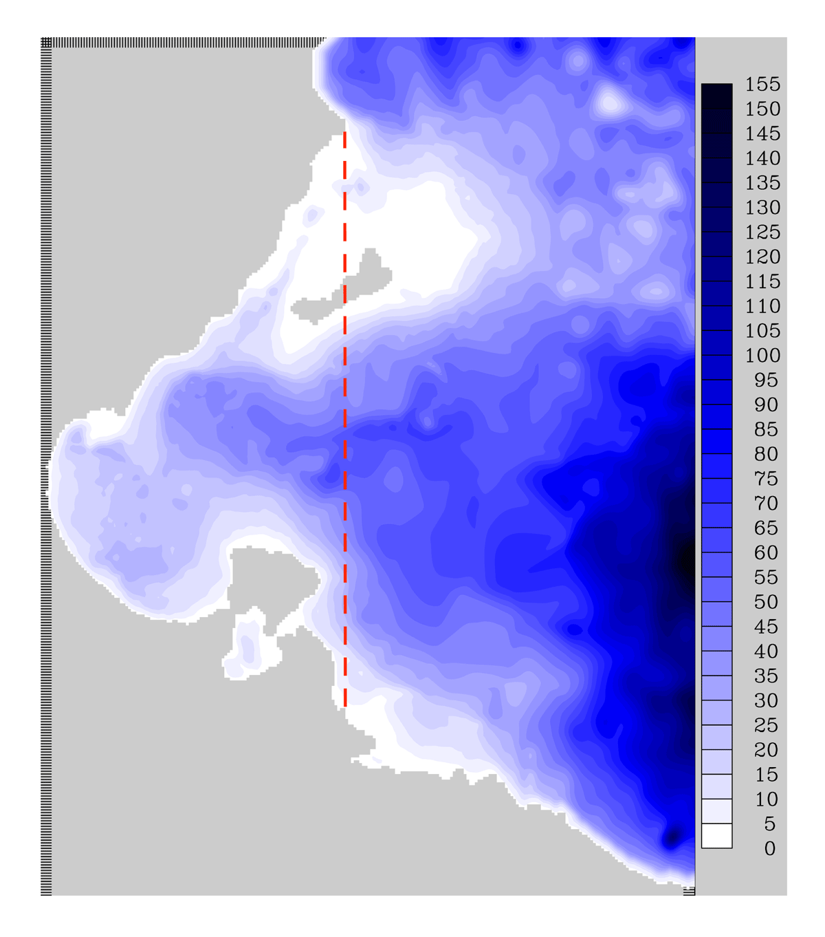
Figure 1
The bathymetry of the model domain. The red dashed line denotes the longitude of the cape Ras Kaboudia at which the trajectories were released to enter the Gulf of Gabès, referred to as the open boundary. Units in m with isobaths every 5 m.
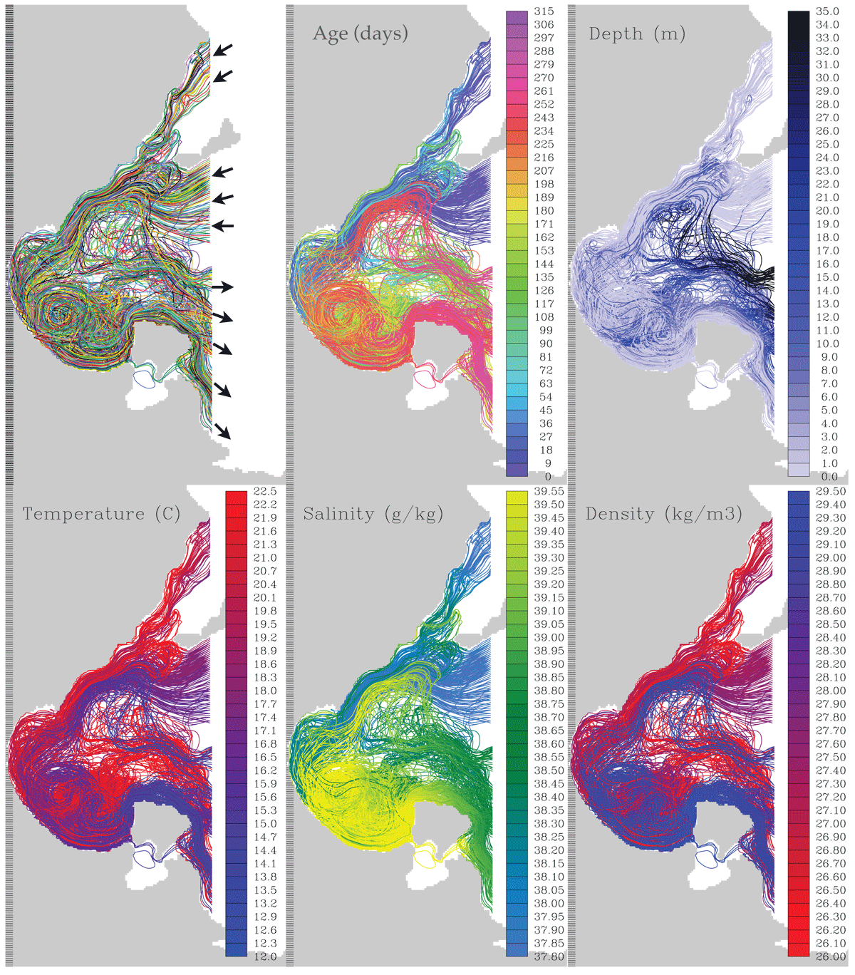
Figure 2
Examples of trajectories entering and exiting the Gulf of Gabès. Colour for individual trajectories as a function of their age, depth, temperature, salinity and density (σ0). Note that this selection of trajectories are longer in time than the average in order to illustrate the circulation of the entire gulf.
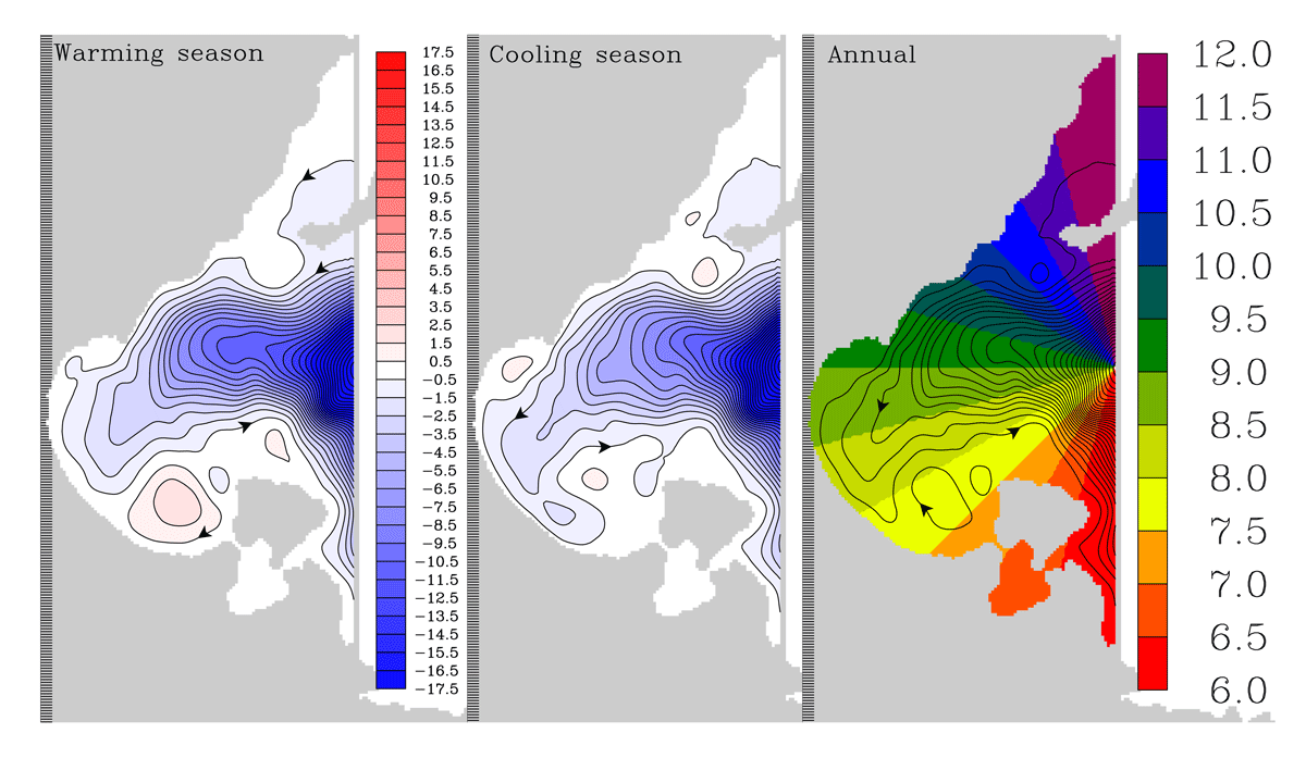
Figure 3
Lagrangian barotropic stream function as a time mean during four years. Left panel: Warming season with trajectories started during January to June, middle panel: Cooling season with trajectories started during July to December, right panel: yearly average with a “clock” division of the Gulf as background that was used to compute the stream functions in Figure 7. Units in mSv, with 1 mSv between the streamlines.
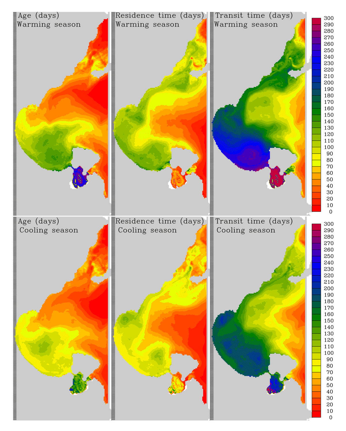
Figure 4
The age (the time to reach a region from the open boundary), residence time (the time flow from a region to the open boundary) and transit time (the sum of the two precedent). Note that the waters are more and more isolated as approaching the southwest. Units in days.
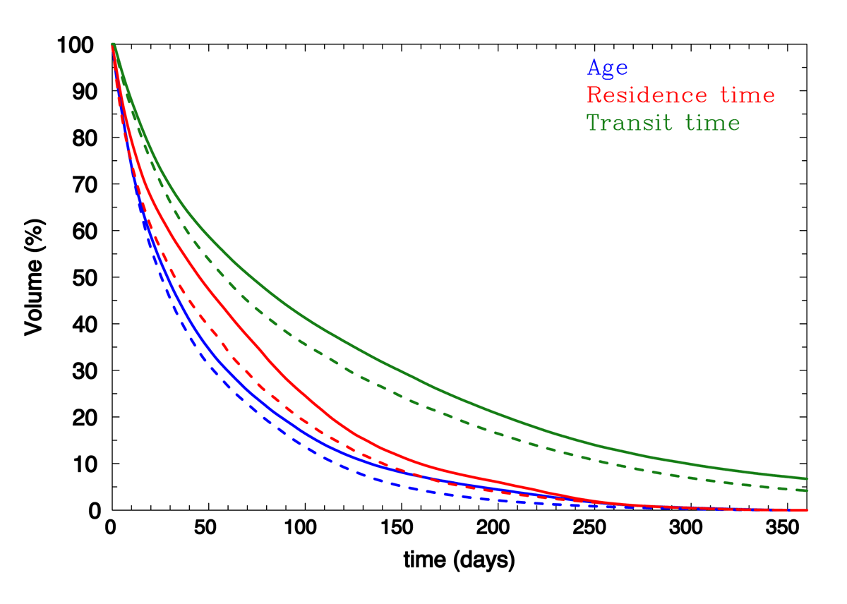
Figure 5
The time evolution of the age in blue, the residence time in red, the transit time defined as the sum of the residence and age in green. Solid lines for the warming season and dashed for the cooling season.
Table 1
e-folding times τ based on the time evolutions of Figure 5. Units in months.
| WARMING SEASON | COOLING SEASON | YEARLY MEAN | |
|---|---|---|---|
| Age | 1.6 | 1.4 | 1.5 |
| Residence time | 2.4 | 1.8 | 2.1 |
| Transit time | 3.9 | 3.2 | 3.6 |
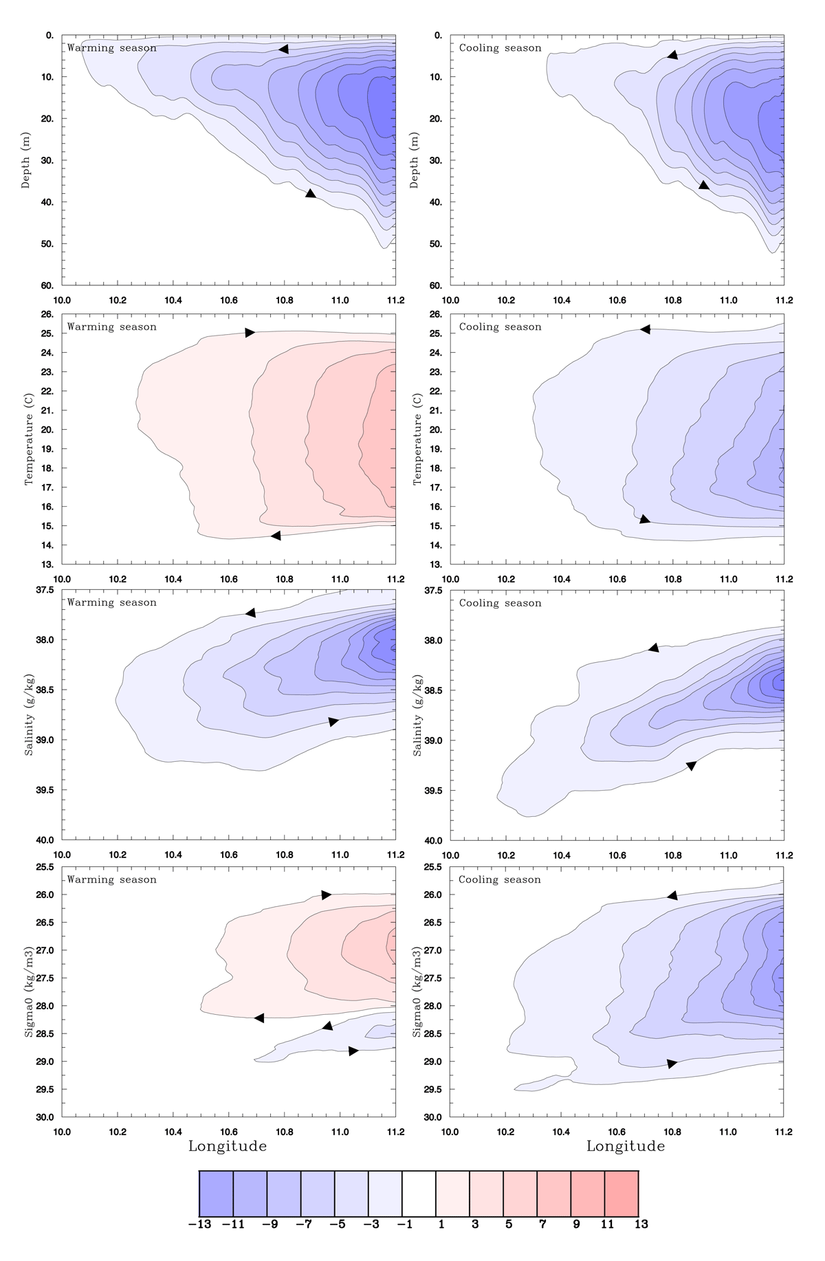
Figure 6
Zonal overturning stream functions as a function of depth, temperature, salinity and density for the warming and cooling seasons. Although these overturning give correct views of the net mass fluxes they tend to exaggerate view of the “vertical” displacements. Units in mSv (1000 m3/s).
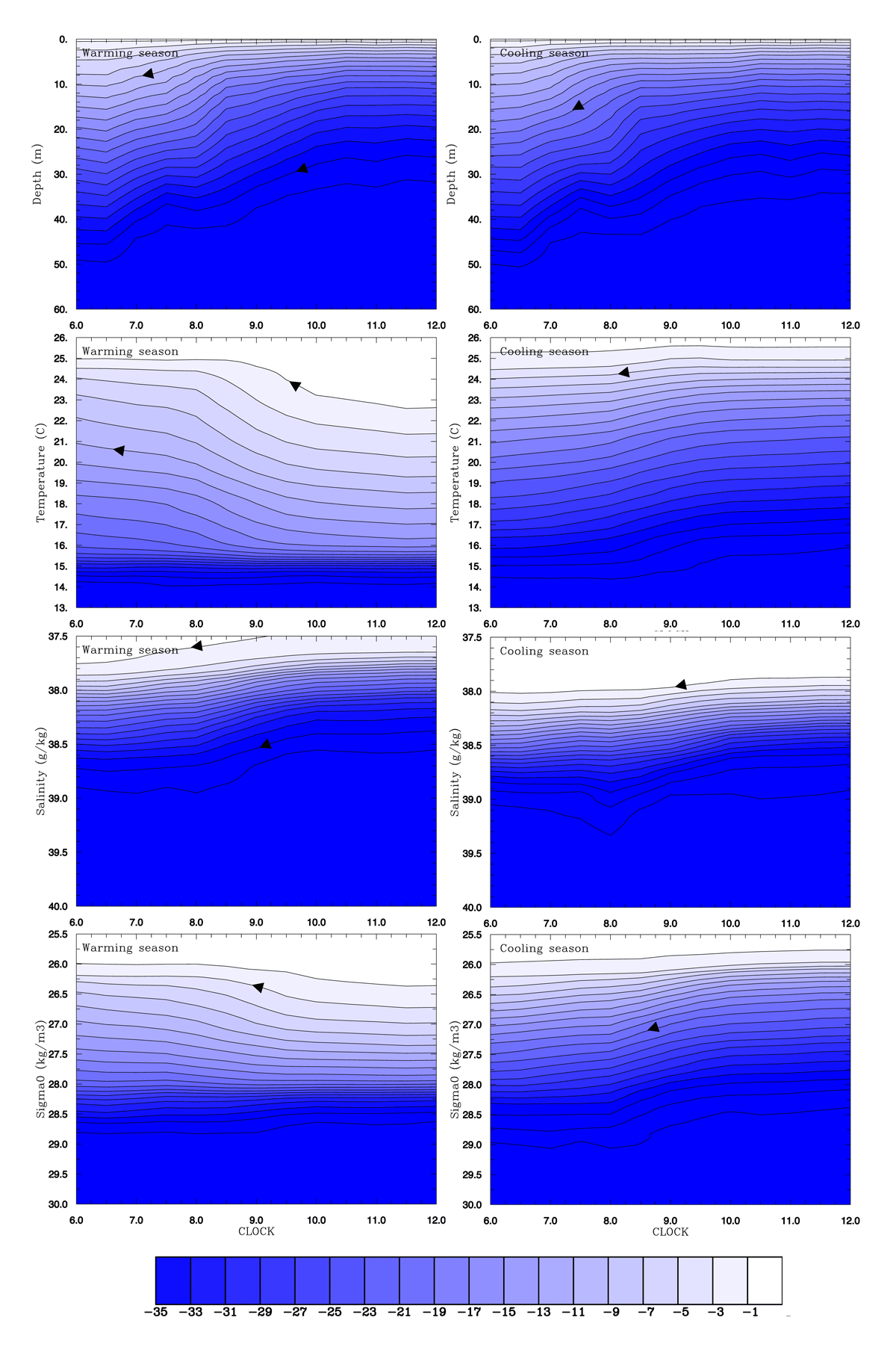
Figure 7
Same as Figure 6 but with the x-axis representing the region defined as a “clock” around the Gulf as shown in the right panel of Figure 3. These stream functions give a more realistic view of the “vertical” displacements compared to the ones in Figure 6.
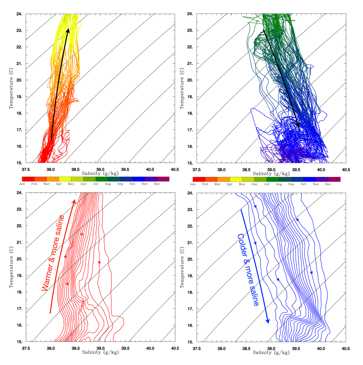
Figure 8
The water mass transformation illustrated by selections of trajectories in the two top panels and the thermohaline stream function for circulation of the Gulf of Gabès in the bottom panels. The “warming season” to the left and “cooling” to the right. Superimposed are isopycnals with intervals of 0.5 kg/m3 ranging from 26.0 to 30.0 kg/m3. The volume transport between two streamlines is 200 m3/s.
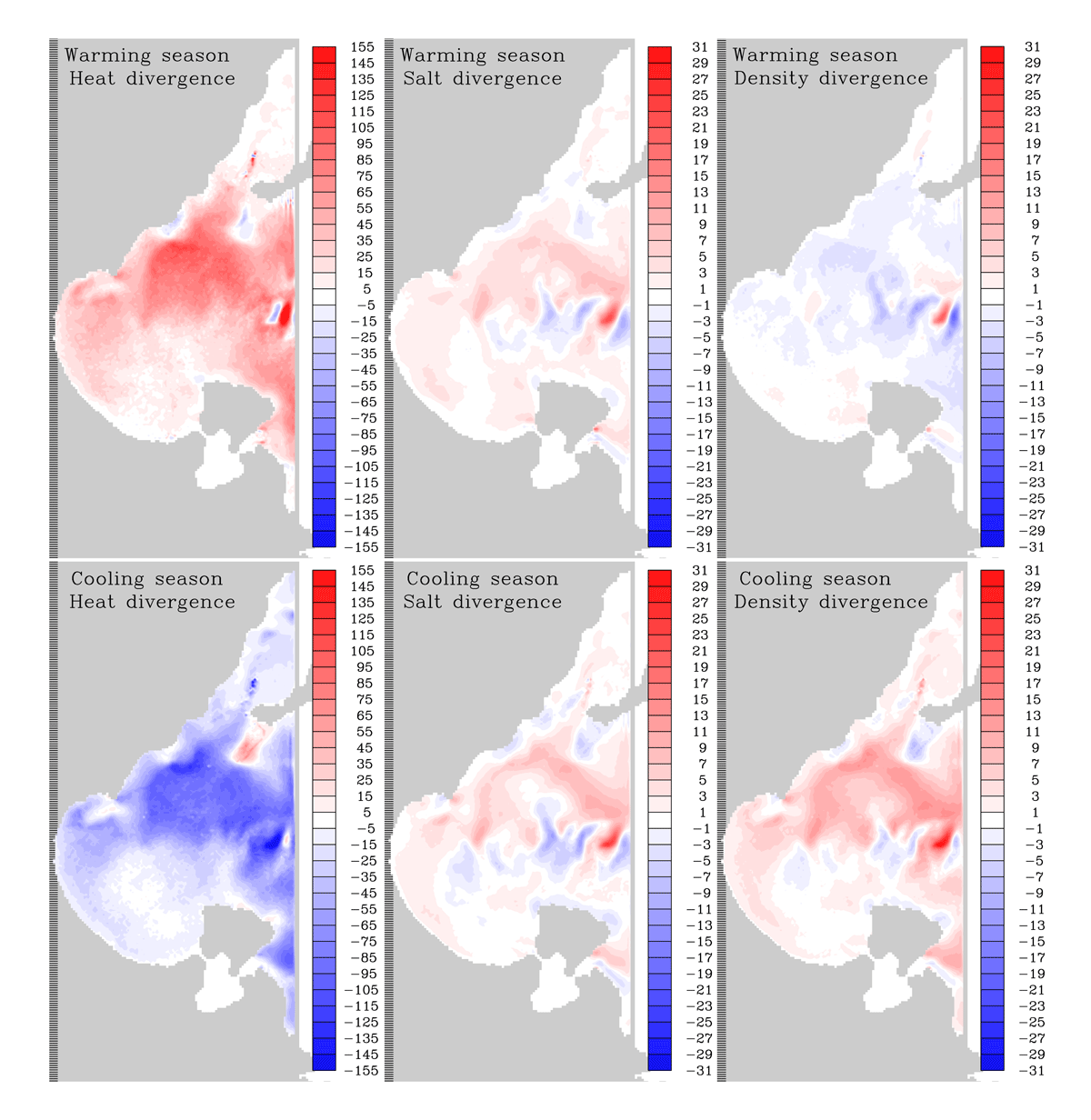
Figure 9
Lagrangian divergence of heat (W/m2), salt kg/(sm2) and density kg/(sm5).
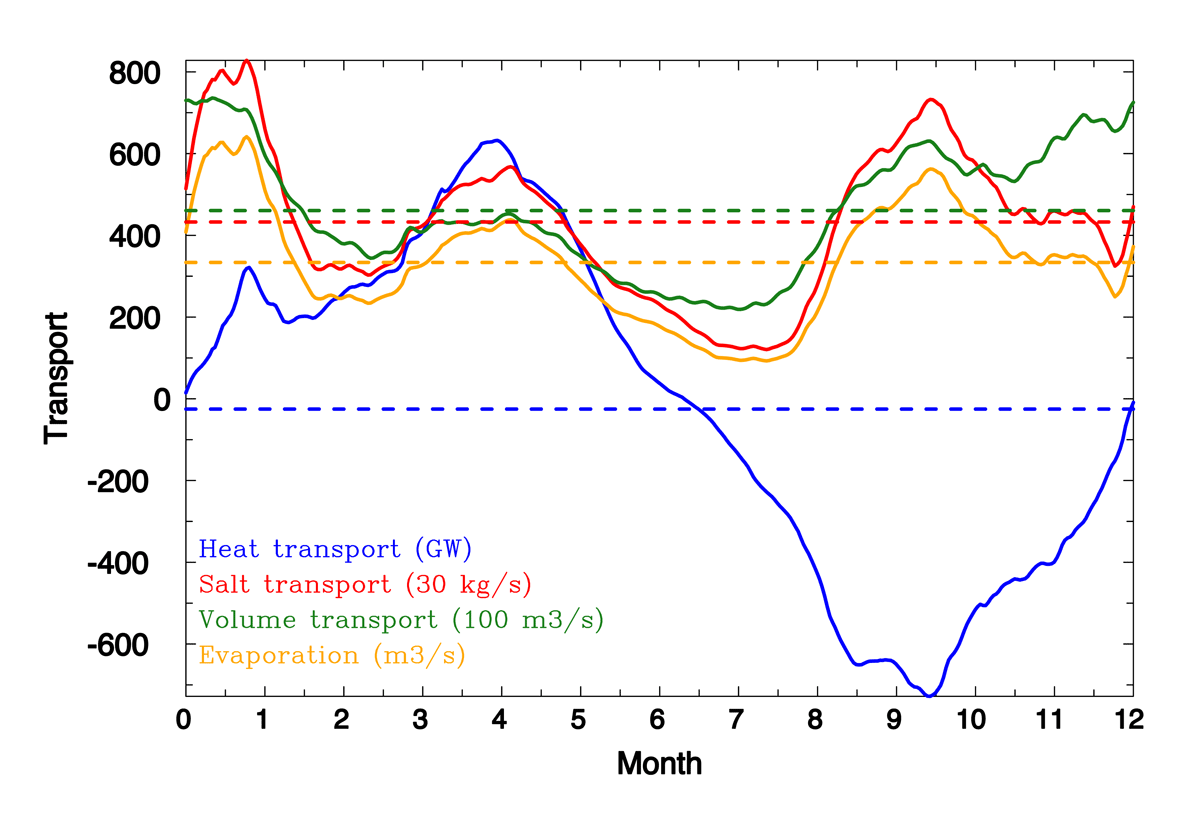
Figure 10
Heat, salt and volume transports through the Gulf of Gabès as a function of time for a mean year. Dashed lines indicate the yearly mean. Units in GW for the heat transport, 30 kg/s for the salt transport and 100 m3/s for the volume transport.
Table 2
The average heat, salt and volume transports through the Gulf of Gabès for the warming and cooling seasons as well as the yearly average based on the evolution in Figure 10. Also the average change of the flow’s temperature, salinity, density and depth.
| WARMING SEASON | COOLING SEASON | YEARLY MEAN | |
|---|---|---|---|
| Heat transport (GW) | 325 | –375 | –25 |
| Salt transport (Mg/s) | 14 | 12 | 13 |
| Evaporation (m3/s) | 365 | 303 | 334 |
| Volume transport (mSv) | 45 | 47 | 46 |
| Temperature change (°C) | 1.7 | –1.8 | –0.1 |
| Salinity change (g/kg) | 0.31 | 0.25 | 0.28 |
| Density change (kg/m3) | –0.21 | 0.68 | 0.24 |
| Depth change (m) | 15. | 14. | 14. |