
1. Introduction
The Gulf of Gabès, situated on the east coast of Tunisia in the Mediterranean Sea, is characterised by a wide shallow continental shelf. According to its physical, biogeochemical and biological characteristics, this Gulf is identified as one of the eleven consensus eco-regions within the Mediterranean (Ayata et al., 2018). The present work of this Gulf should be seen as a case study of a bay, where a number of methods have been applied in order to understand its overturning circulation, water mass transformation and residence times. These methods have been used in other studies for large scale ocean circulation (Berglund et al., 2017; Döös et al., 2012; Speich et al., 2007) but seldom in coastal oceanography. The water deficit in the Mediterranean Sea, due to the excess of evaporation compared to the rates of precipitation and the contributions of river runoff,is compensated by the Atlantic water current that feeds the Mediterranean through the Strait of Gibraltar. At the entrance of the Sicily Channel, the Algerian Current brings the modified Atlantic water, which splits into two branches, one into the Tyrrhenian Sea and the other one into the Sicilian Channel. The latter splits into two veins following separate tracks, one along the southern coast of Sicily and the second along the Tunisian coast with the minimum of salinity (Beranger et al., 2004). This current is called the Atlantic Tunisian Current (ATC), which strength is modulated by the wind and displays strong seasonal variability (Omrani et al., 2016). The Atlantic Tunisian Current splits again into three branches, one of which flows toward the Levantine basin, the second invades the Gulf of Gabès and recirculates cyclonically on the shelf, while the rest becomes a coastal current along the Libyan coast (Ben Jaber et al., 2014; Boukthir et al., 2019). The circulation in this very shallow basin (maximum depth ≈ 150 m at its easternmost limit) is characterised by strong mesoscale variability, with an eddy kinetic energy two-to-three times larger than in the Sicily Channel and Sardinia-Tyrrhenian subregions (Sorgente et al., 2011). It is also known to be resonant for the semi-diurnal tides (Abdennadher, Boukthir, 2006; Sammari et al., 2006). The analysis of baroclinic energy conversion (Sorgente et al., 2011) indicated that this bay is characterised by a permanent energy conversion from eddy available potential energy to eddy kinetic energy. Moreover, it was found that the eddy kinetic energy averaged over the gulf represents about 64 % of the total kinetic energy on an annual mean scale, indicating that the circulation is dominated by fluctuating currents(Boukthir et al., 2019). This could be explained by the abrupt current reversals between the autumn-winter and spring-summer seasons in the southeast of the Gulf. Besides, it was established that the Gulf of Gabès has the highest mean microplastic abundance compared to three other regions in the Mediterranean Sea (Aronikos Gulf, Ligurian Sea and Gulf of Lion) (Tsiaras et al., 2022). The seasonal variation in microplastic distribution between spring and autumn is correlated with significant seasonal variations in surface current circulation (Ben Ismail et al., 2022). The main hydrodynamic processes in the Gulf of Gabès have been identified, but little is known about the transformation of water masses there. Knowledge of the age, residence, and transit times of water masses advected by the Atlantic current is precious for environmental and ecosystem studies. In fact, the cyclonic circulation of the Atlantic Tunisian Current in the Gulf of Gabès, strongly conditions the availability of nutrients and therefore the growth of phytoplankton. The purpose of this work is to study and evaluate the causes of the water mass transformation occurring in the Gulf of Gabès and its associated overturning circulation. The focus will hence be on the mean large-scale circulation and, in particular, how this is separated into warming and cooling seasons. However, the inter-annual variability will not be examined in this study. For this aim, we generated Lagrangian trajectories from the entrance to the Gulf to the exit and investigated how the water’s properties, such as temperature, salinity, and density, change as it flows through it.
The ocean circulation model that has been integrated as well as the trajectory code are described in Section 2 The general horizontal circulation is shown in Section 3. A residence time analysis is performed in Section 4. The overturning and how this needs to be somewhat twisted to get the right view is computed in Section 5. Then, we make a water mass transformation analysis in Section 6. Finally, the study is concluded with a summary and discussion of the main results in Section 7.
2. Modelling the Gulf of Gabès
The modelling of the circulation in the present study is based on the hydrodynamic model ROMS as well as on the mass conserving TRACMASS trajectory model TRACMASS. The analysis throughout this study is grounded on the simulations by these two models.
2.1. The ocean circulation model ROMS
We have used the Regional Ocean Modeling System (ROMS). It is a free-surface terrain-following ocean model that solves the primitive equations based on the Boussinesq and hydrostatic approximations. The equations are solved on a curvilinear grid with a terrain-following vertical coordinate system (Shchepetkin, McWilliams, 2005). The model domain extends from 10°E to 12°E and from 33°N to 35°N as shown in Figure 1. The horizontal resolution was 1/96° (≈ 950 m) in both longitudinal and latitudinal directions. This high-resolution grid mesh of the model allows a good representation of the bathymetry and the large-scale and mesoscale patterns of the circulation. The vertical grid consisted of 25 layers distributed according to the ROMS topographic-following coordinated system. The use of terrain following sigma coordinates is particularly suitable in the Gulf because of its slowly varying topography going from depth of 70 m at its entrance and down to a minimum depth of 2 m near the coast. The model bathymetry is deduced from Smith, Sandwell (1997) topography database by bilinear interpolation onto the model grid. The model was initialised using the MEDATLAS (Fichaut et al., 2003) monthly climatology of observed temperature and salinity fields. Open boundary conditions at the easternmost and northernmost edges of the model domain were prescribed from the monthly outputs (temperature, salinity, sea surface elevation and velocities) of MED12 (Lebeaupin Brossier et al., 2013). The model simulations were forced by wind, atmospheric pressure, heat fluxes, and with tide elevations and currents derived from the barotropic gravity-wave model MOG2D (Roblou, 2004). The model has sponge layers on its north and east open boundaries to prevent the reflection of internal wave energy back into the domain. These regions are excluded from the presentation and analysis of model results. The model was integrated from 1995 to 2007.
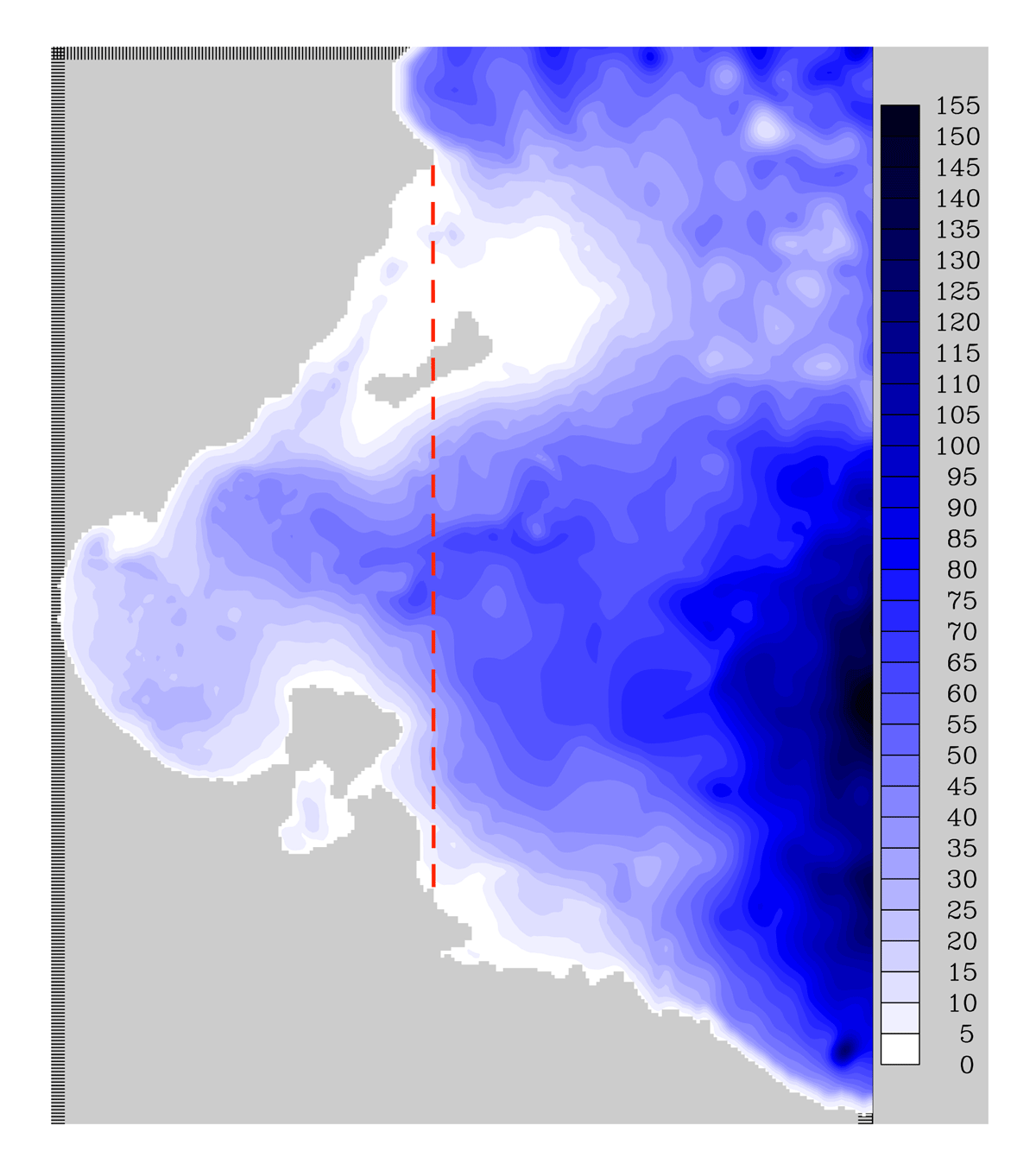
Figure 1
The bathymetry of the model domain. The red dashed line denotes the longitude of the cape Ras Kaboudia at which the trajectories were released to enter the Gulf of Gabès, referred to as the open boundary. Units in m with isobaths every 5 m.
The last 4 years, i.e. 2004 to 2007 of this integration were used in order for the present analysis, i.e. after 9 years of spin-up, which is sufficient for the size and depth of the Gulf of Gabès. For numerical stability, the internal time step is set to 50 s with 30 barotropic intermediate time steps in order to satisfy the CFL stability criteria (Döös et al., 2022).
2.2. The trajectory model TRACMASS and the Lagrangian experiment setup
In the present study, the simulated circulation of the Gulf of Gabès by ROMS has been investigated making use of the trajectory model TRACMASS (Döös et al., 2017). The velocity and mass transport fields were used to compute the Lagrangian trajectories. The TRACMASS scheme is mass conserving and employs mass flux fields (same as volume transport fields if the water is assumed to be incompressible as in ROMS). This makes it possible to calculate a number of quantities that require mass conservation such as Lagrangian stream functions, residence times and water mass transformation in the temperature-salinity space. The TRACMASS code is available on Aldama-Campino et al. (2020).
The Gulf of Gabès was here defined as the region west of the longitude of 11.2°E, which is shown by the red dashed line in Figure 1. This might be somewhat bigger than what is sometimes considered to be the Gulf of Gabès. This definition based on the easternmost point of the Cape of Ras Kaboudia, where the red dashed line ends in the north, makes it possible to define a bay that is secluded. This seclusion makes it possible to calculate quantities such as zonal overturning stream functions since all the water that flows westward into the Gulf through this longitude must eventually exit eastward through the same longitude. This longitude will be referred to as the open boundary, which should not be confused with the open boundary conditions of ROMS located further east and north as described in the previous section. The analysis of the present work is to a large extent based on these simulated trajectories entering the Gulf of Gabès at this open boundary. They were started on all the grid cell walls, which had a westward velocity; once every day during the entire period between 1 January 2004 and 31 December 2006. They were then followed until they exited the Gulf through the same longitude at the open boundary. A total of number of 3,900,659 trajectories were computed and analysed. The mass conserving properties of TRACMASS make it possible to associate a trajectory with a given mass or volume transport it conserves like a tube all along its journey from where it enters until it exits. The n-th trajectory is thus associated with a parcel of a volume transport, computed as the following:
where i, j, k are the longitudinal, latitudinal, and depth indices of the trajectory n. |ui,j,k| is the westward zonal velocity at the longitude at the open boundary where it enters the Gulf; Δy and Δzi,j,k are the meridional and vertical lengths of the associated grid-box wall, respectively. It is this volume transport that is then conserved all along the trajectory due to the mass conserving scheme of TRACMASS (Döös et al., 2017). The temperature and salinity of the trajectory parcel is, however, changing along its journey due to mixing and fluxes through the surface.
A selection of representative trajectories that flow through the Gulf are shown in Figure 2. The trajectory evolution in time, depth, temperature, salinity and density (σ0) is illustrated by their colours. One can already see the basic general circulation of the Gulf from this raw data of trajectories. We will, however, in the following sections analyse the trajectories by computing different quantities that sum over all the trajectories. Two different seasons have been chosen for this. One, which was named the “warming season”, where trajectories have been started between 1 January and 30 June for 2004, 2005 and 2006. The other season, which was named the “cooling season”, where trajectories started between 1 July and 31 December during the same three years. The justification of this definition of a warming and a cooling season will be shown in Section 4 and in Section 6.2. The time mean was computed for these two seasons. It is important to realise that the Lagrangian time mean, which will be used here, is not as simple as the Eulerian one. The Eulerian view is instantaneous, while the Lagrangian one depends on how long a trajectory will take to pass through the studied region, which is here the Gulf of Gabès. The different trajectories will spend different lengths of time in the Gulf, and hence the time mean is not over an exact period of time. Here we have defined it from the time the trajectories start, but one needs to bear in mind that the residence times are all very different for the trajectories, as we will see in Section 4. In case one absolutely needs to relate the Lagrangian time frame to the Eulerian one in the present study, one can, as a thumb rule, delay the Lagrangian by a couple of months (see explanation in section 4), so that January, e.g. corresponds roughly to March or April.
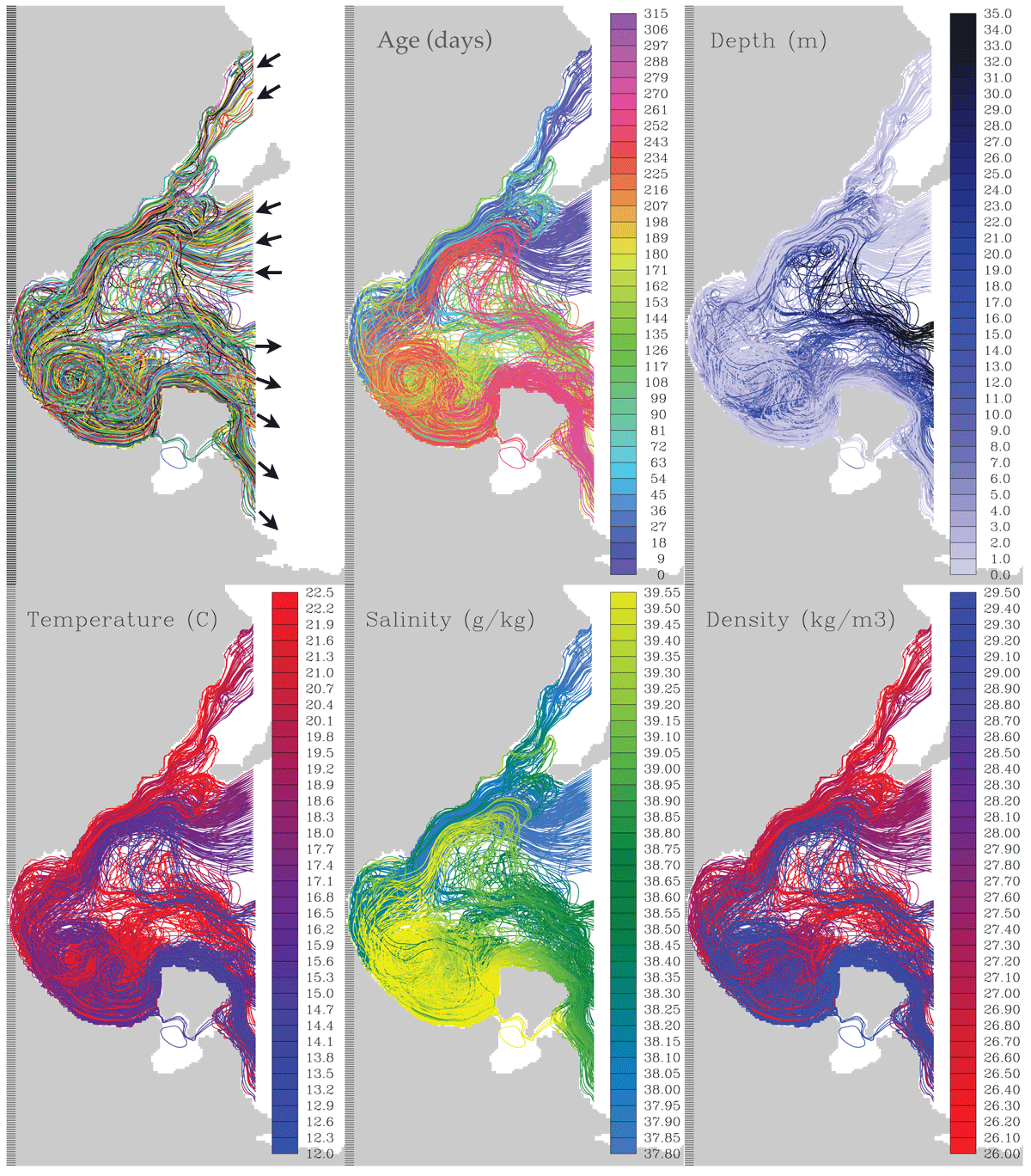
Figure 2
Examples of trajectories entering and exiting the Gulf of Gabès. Colour for individual trajectories as a function of their age, depth, temperature, salinity and density (σ0). Note that this selection of trajectories are longer in time than the average in order to illustrate the circulation of the entire gulf.
3 The horizontal circulation of the Gulf
The selected trajectories of Figure 2 give a first qualitative view of the general horizontal circulation of the Gulf, where the water tends to enter the Gulf in the north and exit in the south. A quantitative analysis requires, however, the ability to sum over the trajectories, which is possible since the TRACMASS simulated trajectories conserve the same mass transport throughout their integrations. The Lagrangian barotropic stream function (Döös et al. 2017; Blanke, Raynaud, 1997) can be computed by summing the volume transport of trajectories vertically and over all trajectories according to
where is the meridional volume transport crossing a constant latitude with the grid index j for the trajectory n. This Lagrangian barotropic stream function can hence be computed by summing the volume transport of all the trajectories over all the vertical levels k and then by integrating from the Tunisian coast and eastward to the open boundary.
There are two main differences between the Eulerian and Lagrangian stream function. The time average for the Eulerian is simple to define over a given period. The drawback is, however, that the flow should strictly be required to be in a steady state, with no temporal variability. This problem is solved with the Lagrangian stream function since it is computed by integrating along the trajectories of the flow from the moment they enter the considered region until they exit and does not require any steady state. This also makes it possible to compute stream functions for chosen trajectories, which e.g. correspond to a particular water mass conversion such as a strong salinification during their journey in the Gulf.
The Lagrangian barotropic stream functions for the warming and cooling seasons are presented in Figure 3. It shows a steady dominant barotropic current entering the Gulf in the northeast and exiting in the southeast filling most of the Gulf except the very south west of Djerba. This depth integrated and time averaged cyclonic circulation is rather constant for the two seasons reaching 28 mSv (1000 m3/s) at its centre on the eastern boundary for the warming season and 30 mSv for the cooling season. There is, however, some strong variability in the south of the Gulf, west of Djerba Island. In this region there is a weak anticyclonic vortex (red contours in Figure 3) we here name the “Djerba Vortex”. The Djerba Vortex is here only visible during the warming season, but is highly unstable and tends to come and go. This southern part of the Gulf is a region with non permanent mesoscale eddies.
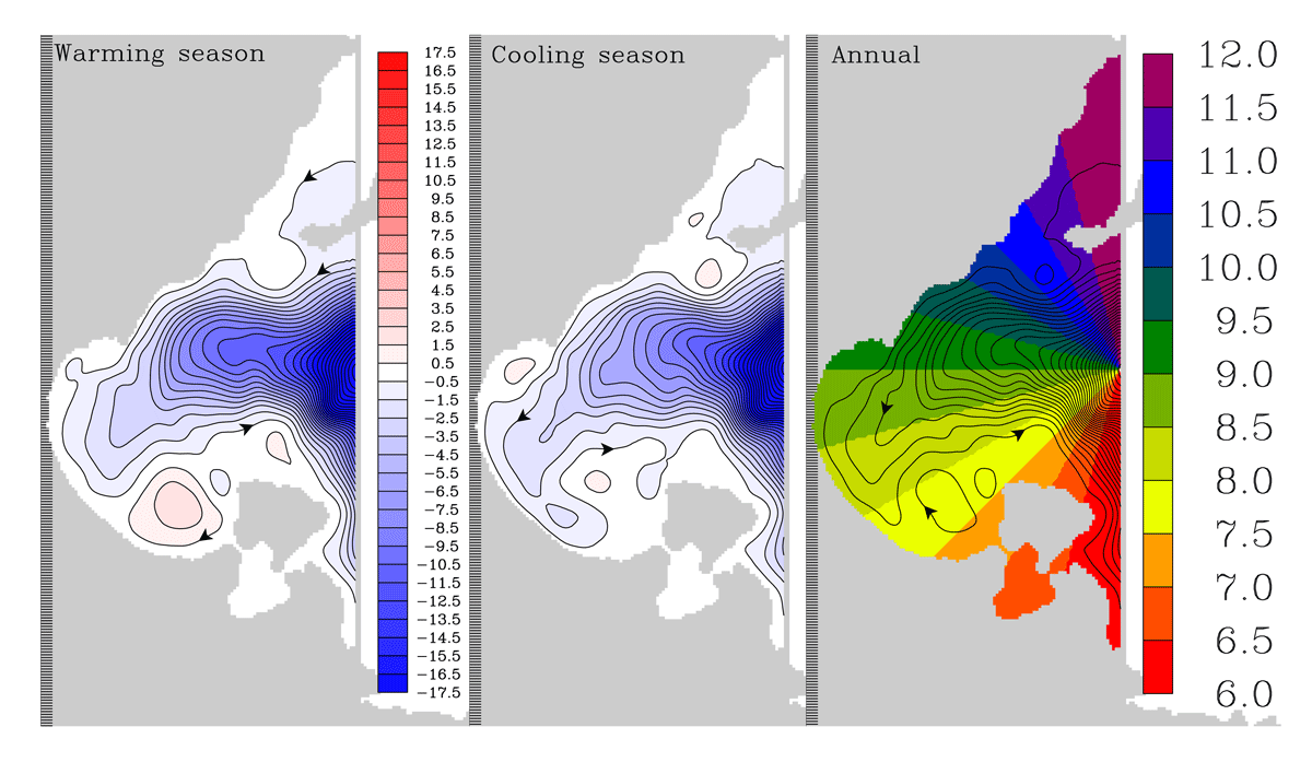
Figure 3
Lagrangian barotropic stream function as a time mean during four years. Left panel: Warming season with trajectories started during January to June, middle panel: Cooling season with trajectories started during July to December, right panel: yearly average with a “clock” division of the Gulf as background that was used to compute the stream functions in Figure 7. Units in mSv, with 1 mSv between the streamlines.
4. The age, the residence and the transit times
The water mass transformation in the Gulf will, to a large extent, depend on how long the water resides in the Gulf. For this we have calculated three quantities related to this time, namely the age, the residence time and the transit time (Dippner et al., 2019). These times, which are all shown in Figure 4 for both the warming season with trajectories released between January and June and for the cooling season, where trajectories have been released between July and December.
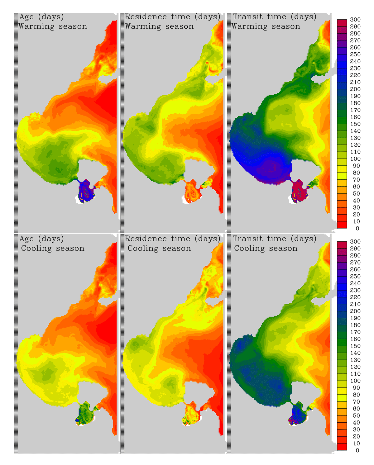
Figure 4
The age (the time to reach a region from the open boundary), residence time (the time flow from a region to the open boundary) and transit time (the sum of the two precedent). Note that the waters are more and more isolated as approaching the southwest. Units in days.
The age of a selection of individual trajectories is shown in one of the panels of Figure 2 by the colours and corresponds to the time they have spent to reach a position from the open boundary (red dashed line in Figure 1), where they were started. The average age, shown in the left panels of Figure 4, is the average time it has taken the trajectories to reach a position from the open boundary of the longitude of Ras Kaboudia (red dashed line in Figure 1), where they were started. The age distribution in the Gulf reveals that the entering waters tend to fill the northern parts within a month or two for both seasons. The southernmost part of the Gulf, on the other hand, is more isolated, and it takes on average about 4 to 5 months to reach this region for the warming season and about one month quicker for the cooling season. This could be explained by the origin of the water in the coastal region of the Gulf. Indeed, during the warming season, the water masses are driven by the Atlantic Tunisian Current crossing the north of the eastern border (surface currents during January to March), while in the cooling season they tend to come from the Libyan coasts and so from the south corner of the border in August-September. That takes a little bit less time to reach the coastal region compared to those driven by the Atlantic Tunisian Current during the winter season.
The residence time, shown in the middle panels of Figure 4, is the time it will take to leave a given position and exit through the open boundary. The structure here is somewhat different from the age along the coast in the north since the water needs to go through the Gulf before exiting. The southernmost part of the Gulf is, however, still isolated and it will take about a 4 to 5 months to exit from here during the warming season and about a month faster for the cooling season. This can be explained by the fact that the water can be trapped in the anticyclonic mesoscale structures that tend to develop during the warming season and create the Djerba Vortex as shown by the red stream function in Figure 3. The exact dynamics of the Djerba Vortex is yet to be determined.
The transit time is the time it takes to go through the Gulf from the open boundary and back, hence the sum of the residence time and the age. It is thus the average time it has taken the trajectories to reach a given position plus the average time it will take until they return to the the open boundary. The transit time is shown in the right panels of Figure 4 and shows that the water is more and more isolated as one approaches the south part of the inner Gulf, just west of the island of Djerba. The longest transit times occur during the warming season (purple in Figure 4) coincide with a region where there tend to be an anticyclonic circulation shown by the red barotropic stream function as in Figure 3.
The age, residence and transit times shown in Figure 4 are averaged over all the trajectories that cross the different grid boxes, which are displayed in the figure as a function of longitude and latitude. In reality, a given water mass does not have one single age, residence and transit time but as many as there are water molecules. This is represented in the present study by water parcels associated with given water volume transports as described by Equation 1. The individual trajectories all take different times to flow through the Gulf. To illustrate this, we have computed the full-time evolution of the age, residence and transit times for the entire Gulf as shown in Figure 5. The residence time evolution is hence how gradually the water in the Gulf will exit and the age how gradually the water will fill the basin. The evolution of these tend to follow rather close e-folding decays that can be expressed by
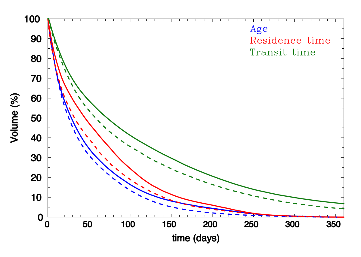
Figure 5
The time evolution of the age in blue, the residence time in red, the transit time defined as the sum of the residence and age in green. Solid lines for the warming season and dashed for the cooling season.
where V(t) is the total volume flow normalised as 100 % at start when the time t = 0. The e-folding time τ is generally set to match V(τ) = 100 e–1 ≈ 37% so it fits with the observed time evolution of the age, residence and transit times at t = τ (Döös et al., 2004). These e-folding times are shown in Table 1 for the two seasons. From Figure 5 and Table 1 it is clear that the cooling season has shorter residence times in the Gulf. This could be due to that the Djerba Vortex tends to exist during the warming season and traps the water in this southern region of the Gulf as shown by the green shading of the age and residence time for the warming season in Figure 4. The shorter age compared to residence time indicates that the Gulf is being filled faster than emptied.
Table 1
e-folding times τ based on the time evolutions of Figure 5. Units in months.
| WARMING SEASON | COOLING SEASON | YEARLY MEAN | |
|---|---|---|---|
| Age | 1.6 | 1.4 | 1.5 |
| Residence time | 2.4 | 1.8 | 2.1 |
| Transit time | 3.9 | 3.2 | 3.6 |
5 The overturning circulation of the Gulf
The overturning circulation in the Gulf of Gabès can, to a large extent, be summarised as fresher surface waters entering from the northeast and exiting in the southeast as deep and more saline waters. This overturning circulation has here been calculated with Lagrangian zonal overturning stream functions. They have been computed by summing the zonal volume transports associated with the trajectories that flow through the Gulf. The trajectories are thus initiated at the longitude of Ras Kaboudia and followed until they exit again through the same longitude. The integration of the zonal transports is first over the latitude indices j and then from the bottom of the ocean and up as follows:
where is the zonal volume transport crossing a constant longitude with the grid index i for the trajectory n.
This zonal overturning is shown in the Figure 6.
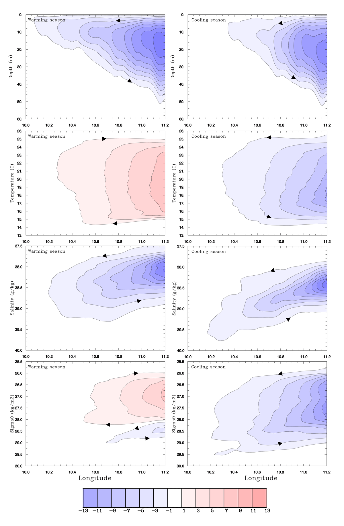
Figure 6
Zonal overturning stream functions as a function of depth, temperature, salinity and density for the warming and cooling seasons. Although these overturning give correct views of the net mass fluxes they tend to exaggerate view of the “vertical” displacements. Units in mSv (1000 m3/s).
In Eq. 4 the depth coordinate of the flux can be replaced by a tracer, such as temperature, salinity or density as follows:
Here Ω stands for the temperature, salinity or density. The index m can be an isothermal, isohaline or isopycnal surface, depending on the selection of tracer. The Lagrangian zonal overturning stream functions that are shown in Figure 6 have on the vertical axes the depth, temperature, salinity and density. They have been computed separately for the warming and cooling seasons. These seasons are only defined when the trajectories are released. There is, hence, a lag of a few months on average due to the residence time before they exit (see previous section). This in order to separate the circulation into a cooling and a warming season since they tend to have rather different dynamics.
This is clearly viewed by the stream function as a function of temperature in Figure 6, where the water is entering as colder water than at the exit for the warming season and the opposite for the cooling one. The overturning as a function of depth is, in contrast, rather similar for the two seasons, but with waters reaching further west into the Gulf during the “warming season”. When using salinity as a “vertical” axis, it shows that there is a distinct salinification in the Gulf during both seasons. This salinity overturning is a result of the fresher Atlantic Tunisian Current entering the Gulf in the north and gradually becoming more and more saline as it flows deeper in the Gulf. When the water turns back eastward, it mixes with the fresher water outside the Gulf and becomes fresher again, but not as fresh as when it entered the Gulf. This explains the sloping streamlines in the zonal direction, both as the flow is westward and eastward, as shown by the arrows on the streamlines in Figure 6.
The zonal stream function as a function of density (bottom panels of Figure 6) shows the combined effect of temperature and salinity on the water, with a rather weak stream function during the warming season with denser water entering than exiting. The cooling season, on the other hand, has a strong overturning with the reverse effect with a densification of the water as it flows through the Gulf.
The disadvantage of these zonal stream functions is that the stream lines tend to give an exaggerated vertical displacement, which is due to the meridional summing of west- and eastward flowing waters. The same hold true for when the temperature, salinity and density are used as a vertical coordinate. A stream line from a stream function is in fact not the same as a trajectory unless the flow is 2D and in steady state. Here neither is true. A known case for this is the Deacon Cell in the Southern Ocean, where water appears to flow from the surface to the deep ocean in the overturning stream function, which in fact is not the case (Döös, Webb, 1994). To get around this, we have divided the Gulf into 12 slices, as shown in the right panel of Figure 3. Each coloured slice has been defined like the half hours of a clock, from 6 to 12. A division method that has been used to study the North Atlantic Subtropical Gyre (Berglund et al., 2022). The overturning stream functions have then been computed for this circular coordinate as an x-axis, as shown in Figure 7. The left at 6 “o’clock” on the x-axis corresponds to where the trajectories leave the Gulf in the southeast and the 12 “o’clock” to where they enter in the northeast. This overturning stream function has the advantage that the east- and westward flowing waters are not cancelling each other. The flow is hence more like the one in a channel that turns around in a half circle, which is the horizontal circulation in the Gulf as illustrated by the stream lines of the barotropic stream function (Figure 7). The stream lines in Figure 6 that seem to flow westward into the Gulf at the surface and return out eastward at 50 m depth give a false impression of a deep overturning. We can now see in this projection of Figure 7 that instead the water is deepening on average by only about 14 m.
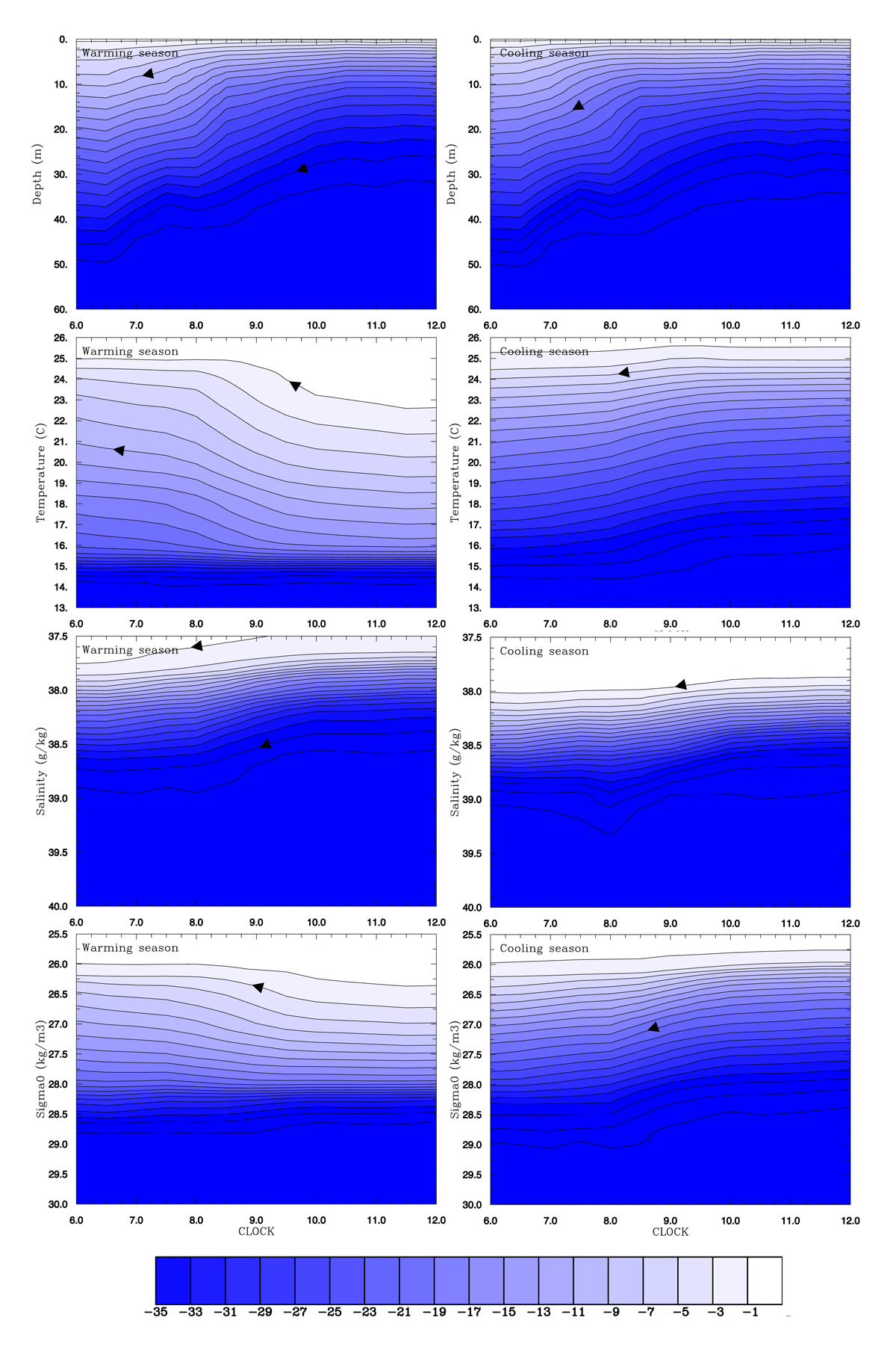
Figure 7
Same as Figure 6 but with the x-axis representing the region defined as a “clock” around the Gulf as shown in the right panel of Figure 3. These stream functions give a more realistic view of the “vertical” displacements compared to the ones in Figure 6.
The water tends to reach the highest salinities when it flows through the innermost part of the Gulf in the southwest region. This explains the “dip” on the streamlines at 8 “o’clock” in the stream function as a function of salinity during the cooling season in Figure 7.
6 The water mass transformation
As the water flows through the Gulf, it will gradually change its temperature and salinity by mixing and through heat exchange with the atmosphere, as well as the fresh water flux through the sea surface due to Evaporation–Precipitation. This change of the water’s temperature and salinity can be referred to as a “water mass transformation” (Groeskamp et al., 2019).
6.1 The thermohaline view
The water mass transformation can be directly seen by tracing a selection of trajectories in the T-S (temperature-salinity) space, as shown in the top panels of Figure 8. The choice of these trajectories was made so that they are rather “long” in the sense that they will take at least 5 months and also undergo a temperature change between 15 to 25°C. This is in order to illustrate the full warming and cooling seasons. The net effect has been computed by summing over all the trajectories that undergo this warming or cooling in the T-S space in order to construct thermohaline stream functions (Döös et al., 2012; Berglund et al., 2017), which are shown in the bottom panels of Figure 8. The stream lines show here the net quantitative diathermal and diahaline flow with a volume transport of 200 m3/s between each pair of stream lines. The trajectories during the warming season show a rather smooth gradual warming and salinification, which is also well illustrated by the corresponding stream function in red.
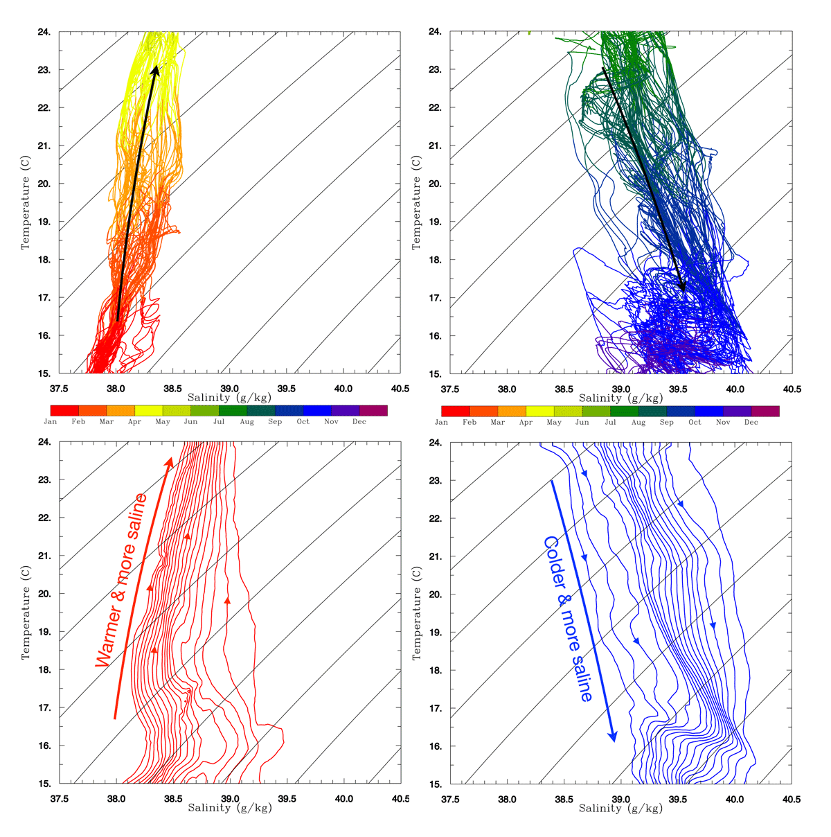
Figure 8
The water mass transformation illustrated by selections of trajectories in the two top panels and the thermohaline stream function for circulation of the Gulf of Gabès in the bottom panels. The “warming season” to the left and “cooling” to the right. Superimposed are isopycnals with intervals of 0.5 kg/m3 ranging from 26.0 to 30.0 kg/m3. The volume transport between two streamlines is 200 m3/s.
The equivalent for the cooling season is somewhat different in the sense that the trajectories tend to oscillate in the salinity space as they are cooling. This oscillation is to some extent smoothed out when summing over the trajectories in the stream function, as shown by the blue stream lines in Figure 8. Even the corresponding stream function in blue shows some of this oscillation, even though it’s much smoother than the individual trajectories. The cause of these oscillations during the cooling season remains to be studied. For both seasons, the thermohaline stream function is diapycnal (Figure 8) therefore arising from mixing process.
6.2 Lagrangian heat and salt divergence
A total budget of the water mass transformation of all the water flowing through the Gulf for the entire period with no selection of trajectories is, however, needed. This has here been quantified by computing the rate of change the trajectories undergo when they pass through each model grid box, following a method developed by Berglund et al. (2017). The aim of this is to compute the rate of change of heat and salt per unit area from the trajectories. This makes it possible to locate the most important geographical areas of heating/cooling and salinification/freshening. When a trajectory travels through a grid box it will change its temperature and salinity due to mixing and also due to exchange with the atmosphere if in the surface layer. The heat gain or loss of a given trajectory can then be computed by taking the temperature the trajectory has when it leaves the box minus the temperature it had when it entered. The trajectories’ temperatures and salinities have been saved for each grid wall passing. The divergence of the heat, salt and density fluxes in a given horizontal grid box are:
Here, Fn is the volume transport of a nth trajectory expressed by Eq. 1, which is conserved all along its journey from where it enters the Gulf until it exits. and are the temperature and salinity a trajectory has as it enters the grid box i,j,k, and and are the temperature and salinity the trajectory has when it leaves the same grid box. cp = 4001 J kg–1 °C–1 is the sea water specific heat and ρ0 = 1026 kg m–3 is ROM’s Boussinesq reference density. i,j,k is the grid box the trajectory passes through and is set by the trajectory’s position in x, y and z respectively. Note here that this integral includes all trajectories flowing in and out of the entire water column and thus sums over the vertical indices k so that the divergences only here depend on the horizontal indices i and j. Q is thus the heat, salt and density divergences expressed in W/m2, kg/(sm2) and kg/(sm2) respectively. A region of positive heat divergence implies that the trajectories are taking up heat and since the trajectories pass through the grid box on a much shorter time scale than the seasonal variability of the temperature of the water. In the present study, we are summing over all the trajectories, and even though the individual trajectories will exchange heat and salt with each other; the total sum has to come from the atmosphere since we are integrating over the entire water column. A positive salt divergence implies similarly an equivalent salt flux from the atmosphere, which corresponds in fact to a net evaporation.
These divergences have been computed separately for the “warming” and “cooling” seasons as shown by Figure 9. Note once more that the seasons are only defined when the trajectories are released and that they tend to take several months before exiting, as we saw in the previous section. The salt divergence dominates in most parts of the Gulf, but there is a region in the middle south, where it is negative. This region corresponds to the exiting saline water, which is strongly mixed with the fresher water from the rest of the Mediterranean and creates a region of meandering mixing between two water masses. This also shows up in the density divergence and is due to the mixing of salt since it is not visible in the heat divergence.
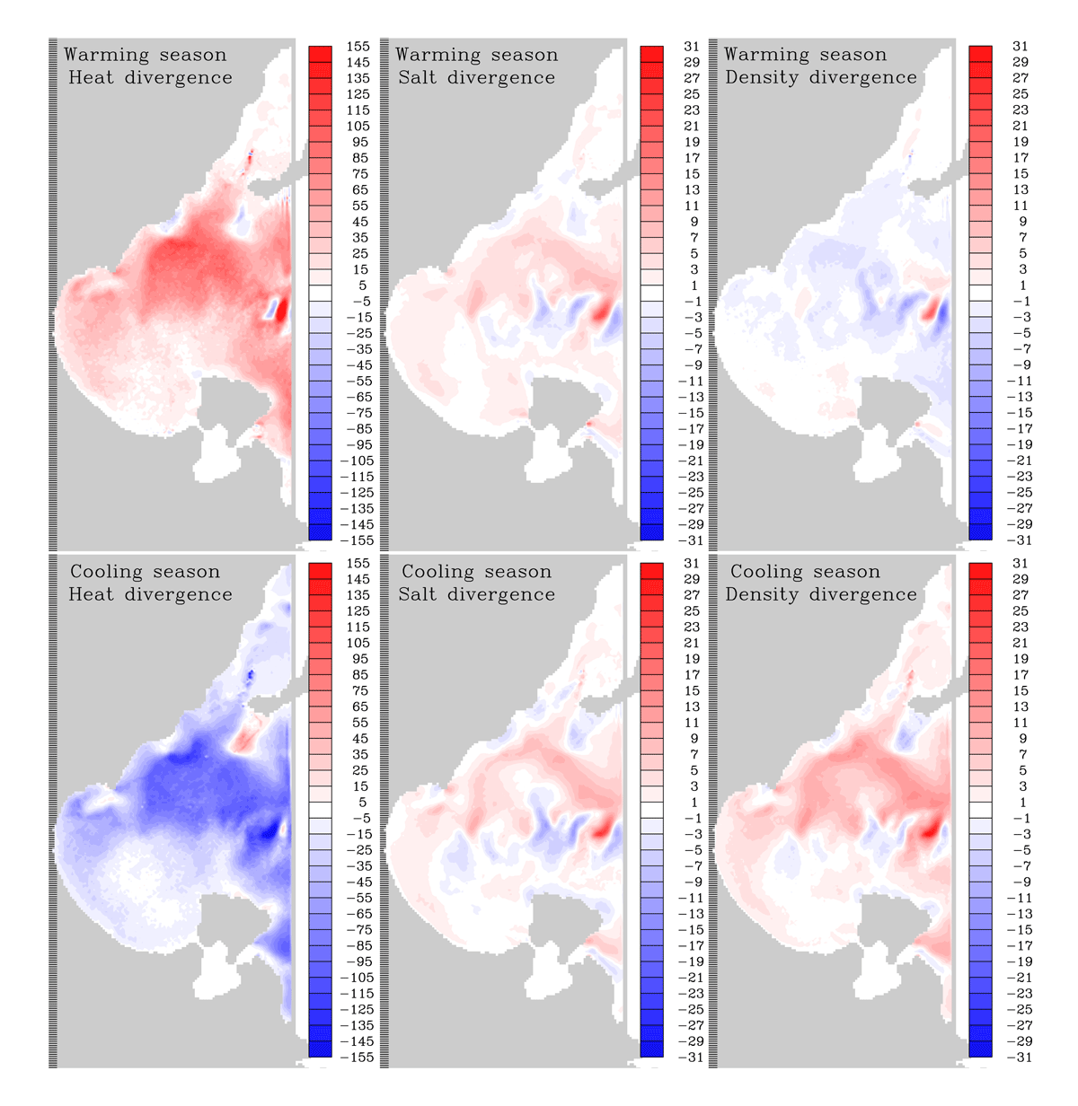
Figure 9
Lagrangian divergence of heat (W/m2), salt kg/(sm2) and density kg/(sm5).
A total heat and salt transports into the entire Gulf expressed in W and kg/s of salt can be computed by only considering the temperatures and salinities of the trajectories when they enter and exit. This hence measures the total change of the flow through the Gulf and is defined as
where this time and are the temperature and salinity of a given trajectory as it enters the Gulf and and are the temperature and salinity of the same trajectory when it leaves the Gulf. These total heat and salt transports have been computed as an average year based on the trajectories that were initiated between 1 January 2004 and 31 December 2006. They are presented together with the total volume flux associated with these trajectories and hence the volume flux passing through the Gulf in Figure 10. The heat transport through the Gulf evens out between the warming and cooling seasons with close to zero net yearly heat transport. Hence our definition of a warming season for trajectories that were started during 1 January and 30 June and a cooling season for trajectories started during 1 July to 31 December were justified. This is because the seasonal lag of the water temperature and the transit time compensate each other. This can be understood by considering a typical trajectory that starts 1 January and exits 1 April. It will first cool down for two months until the end of February and then warm up for two months so it reaches the same temperature when it exits the Gulf as it had when it entered the Gulf. This explains why the heat transport is close to zero at the beginning of the year (blue curve in Figure 10). This also explains the seasonal sign change of the zonal overturning cell as a function of temperature in Figure 6 with a net export of heat out of the Gulf during the heating season and a net import during the cooling season. The net salt transport into the Gulf that has been computed with Equation 8 and shown by the red curve in Figure 10 is in fact the “equivalent” salt transport, which in fact corresponds to a fresh water flux through the sea surface. This can be understood by following the water parcel of a typical trajectory that enters the basin with the volume transport F and the salinity Sin and exits with the salinity Sout. The trajectory will increase its salinity due to the net evaporation E, which corresponds to an increase of the trajectories salt flux of ESin. The salt flux out is thus F Sout ≈ F Sin + E Sin. The net evaporation estimation is hence
which is illustrated by the yellow curve in Figure 10. It closely follows the salt divergence and would only deviate if the salinity itself would strongly fluctuate, which is rarely the case in non-brackish seas. The temporal evolution of salt transport and the associated evaporation is to a large extent in phase with the volume transport except for trajectories started during November and December. Note that this computation of the net evaporation by Eq. 9 neglects the effect of the variability of total salt content of the Gulf and is delayed in time compared to the instantaneous Eulerian computation of the net evaporation.
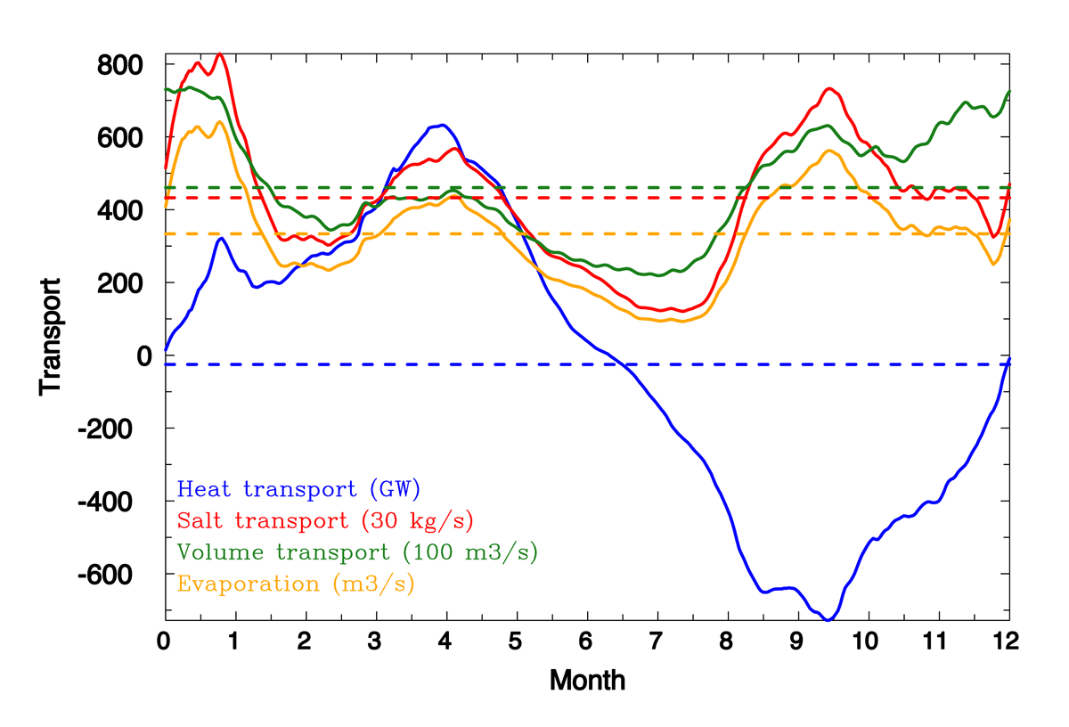
Figure 10
Heat, salt and volume transports through the Gulf of Gabès as a function of time for a mean year. Dashed lines indicate the yearly mean. Units in GW for the heat transport, 30 kg/s for the salt transport and 100 m3/s for the volume transport.
The trajectories will change their salinity as they flow through the Gulf due to mixing and evaporation. On a yearly mean, there is a net salinification of 0.28 g/kg, which is due to net evaporation that corresponds to an equivalent net salt transport of 13 Mg/s (103 kg/s) of salt (Table 2). There is, however, no real net salt transport into the Gulf since it is assumed that the total amount of salt is in a steady state. There is, as shown by the red curve in Figure 10, a strong seasonal variability, which closely follows the water volume influx variability. The salinification together with the cooling makes the water denser with 0.68 kg/m3 during the cooling season, when the water becomes in average 1.8°C colder (Table 2). The salinification is, however, not enough to make the water denser during the warming season, when the water instead becomes 0.21 kg/m3 less dense.
Table 2
The average heat, salt and volume transports through the Gulf of Gabès for the warming and cooling seasons as well as the yearly average based on the evolution in Figure 10. Also the average change of the flow’s temperature, salinity, density and depth.
| WARMING SEASON | COOLING SEASON | YEARLY MEAN | |
|---|---|---|---|
| Heat transport (GW) | 325 | –375 | –25 |
| Salt transport (Mg/s) | 14 | 12 | 13 |
| Evaporation (m3/s) | 365 | 303 | 334 |
| Volume transport (mSv) | 45 | 47 | 46 |
| Temperature change (°C) | 1.7 | –1.8 | –0.1 |
| Salinity change (g/kg) | 0.31 | 0.25 | 0.28 |
| Density change (kg/m3) | –0.21 | 0.68 | 0.24 |
| Depth change (m) | 15. | 14. | 14. |
7. Summary and discussion
The present study of the Gulf of Gabès has demonstrated how water mass transformation can be estimated from a Lagrangian perspective, wherein the water gradually changes its characteristics while flowing through the bay. Several parameters have been calculated, including age, residence and transit times, as well as various overturning stream functions, to describe and quantify the water mass transformation in the Gulf. Detailed mapping of residence times can also provide valuable insights into how coastal pollution persists within the bay before dispersing and impacting the wider Mediterranean region. One of the objectives of this study was to identify the water mass transformation of the cyclonic current that circulates along the coast throughout the Gulf. Specifically, the transformation of the relatively fresh Atlantic Tunisian Current, which contributes to this water mass, through processes like mixing and evaporation into the more saline waters of the Mediterranean. The majority of water transits through the Gulf within three months (Table 1), allowing it to adjust to seasonal changes in temperature and salinity. This justified our definitions of a “warming season” for trajectories initiated between January and June and a “cooling season” for trajectories initiated between July and December.
The Gulf provides a good example of how an overturning stream function can present an exaggerated depiction of deep water formations. The streamlines illustrated in Figure 6, which appear to flow westward into the Gulf at the surface and eastward at a depth of 50 m, create a misleading impression of a deep overturning circulation. To address this issue, we adopted an alternative approach by dividing the Gulf into curved “slices,” resembling the divisions of a clock, where each slice corresponds to a specific “hour” (as shown in the right panel of Figure 3). This alternative representation of the horizontal coordinate revealed an average deepening of only about 14 m and provided a more realistic overturning in the temperature, salinity and density space (Figure 7).
The mean 3D circulation can be viewed as a half-spiral, where the westward entering water in the north is shallower, fresher and lighter than the eastward exiting waters in the south. This deepening is largely attributed to the salinification within the Gulf, with a salinity increase of 0.28 g/kg, resulting from the dominance of evaporation over precipitation and river runoff throughout the year. However, it is worth noting that the effect on water density variability is presumably due to temperature variations, whose impact prevails over that of salinity variations. The analysis of representative trajectories and their associated Lagrangian thermohaline stream function (Figure 8) revealed that mixing within the Gulf occurs through diapycnal processes during both seasons. Using the Lagrangian divergence thus connects the Lagrangian thermohaline stream function to geographical space, increasing our understanding of the overturning circulation in the Gulf. If the spatial distribution of heat flux divergence is globally homogeneous in the Gulf, the salt divergence is not. There is a region in the middle south, where the signs of salt divergence change for both seasons. This region corresponds to the exit of saline water, which is strongly mixed with the fresh water and creates a region of meandering mixing between two water masses. Density divergence is predominantly negative (positive) nearly everywhere during the warming (cooling) season, except for the southernmost region just west of Djerba, where no significant changes were detected. This region is characterised not only by the oldest water in terms of age but also by a longer residence time, taking almost 4 months or more during the warming season to leave this inner part of the Gulf. These factors have severe implications for industrial pollution released into the Gulf of Gabès, making it one of the most polluted regions in the Mediterranean. Finally, it is worth noting that, on yearly and spatial means, the volume transport associated to this overturning is approximately 46 mSv (Table 2). This overturning occurs during both seasons and equalises the heat transport through the Gulf between the warming and cooling seasons, resulting in no net yearly heat transport (Figure 10). Unanswered questions that could be addressed in future similar studies using the same modelling tools could e.g. be the inter-annual variability and more detailed studies of the currents in the Gulf. Downscaling and modelling of the circulation in the Gulf based on climate scenarios are also possible. The scenarios show a projected drier climate, which should lead to an even stronger salinification in the Gulf and thus affect the circulation and water mass transformation in the future. The current Lagrangian approach can be applied to any gulf, bay, or ocean basin that exhibits a secluded circulation pattern following the coastline, such as the Gulf of Mexico, the Weddell Sea, or the Gulf of Tunis.
Acknowledgements
The Lagrangian trajectory model TRACMASS v7.0 can be downloaded from 10.5281/zenodo.4337926 Aldama-Campino et al. (2020). The authors would like to thank Dr. Slim Gana for providing help throughout the work.
Funding Information
This work has been financially supported by the Swedish Research Council through grant agreement no. 2019-03574. The authors Moncef Boukthir and Abdennadher Jihene are supported by the Ministère de l’enseignement supérieur through the Materials and Fluid Laboratory.
Competing Interests
The authors have no competing interests to declare.