
1. Introduction
Cold events in wintertime have been widely noticed by both of scholars, media, and the public people in China, because they have great impacts on the socioeconomy, health, and even human lives (Liu, 1990; Ding et al., 2008; Peng and Bueh, 2011). For example, in 2008, a special cold event coupled with heavy rain, snow and icy conditions swept most of China, affecting all the sectors and aspects of people’s lives thereof and inducing large amount of economic loss at the same time (Zhao et al., 2008; Wang et al., 2008; Hong et al., 2009). Besides, there are still other widespread cold events brought rain, storms and decreased temperatures in Northeast and North China, leading to severe and persistent weather-related disasters (Sun and Zhao, 2010; Liu et al., 2018; Qin and Li, 2020).
Previous studies have focused on the features and the reasons for the occurrence and development of cold events from different kinds of aspects like the case studies, annual changes, and decadal variations, and tried to build up connection to the typical systems like winter monsoon, East Asian trough, and upper-level westerlies et al. (Gong and Ho, 2002; Xue and Zhang, 2017; Liu et al., 2020; Zhang et al., 2022). In addition, external forcings like sea surface temperature (SST) and Arctic sea ice melting are utilized for the analysis the reasons for changes of cold events. Jiang et al. (2014) said the SST anomalies in the tropical Pacific and Atlantic are related to the interannual temperature anomalies in Northeast China. The abnormal Arctic sea-ice, snow cover over the Mongolian Plateau have been found to be related to interdecadal changes in temperature over Northeast China (Liu and Zhu, 2020; Xue et al., 2022). However, little attention has been paid to the variability of cold events on subseasonal time scales, and the underlying causes are unclear.
Madden-Julian Oscillation is a tropical large-scale oscillation with a subseasonal periodicity (Madden and Julian, 1971; 1994). The MJO is originated from the tropics and incites local convection and precipitation in different tropical regions. But, it has also a significant impact on the extratropical atmospheric circulation, and further contributions to synoptic to subseasonal weather predictions (Waliser et al., 2003; Matthews et al., 2004). During the whole life cycle of the MJO, the related tropical convective activities could bring about the source signals that affect the midlatitude atmospheric variability via the propagation of Rossby wave (Ferranti et al., 1990; Kim et al., 2006; Park et al., 2010; Liu and Hsu, 2019; Kim et al., 2020). It found that when the MJO reaches the state of 2 to 4 phases the whole China will experience the cooling temperature anomalies. This cooling process is highly related to a dipole connection associated with phase 7 of the MJO (Kim et al., 2020). Regarding the possible physical mechanism in dynamics and thermodynamics, many studies have also discussed previously (Zhang et al., 2020; Jiang et al., 2020; Kim and Zhang, 2021; Rostami et al., 2022; Jeong et al., 2015). For example, during the cold extreme event in 2008, the northerly winds related to MJO convections have been maintained for a longer time suggesting the effects of tropical atmospheric variability [30]. Meanwhile, when the MJO-related convection propagates northeastward to midlatitudes, the incited Rossby wave anomalies can modulate the atmospheric circulation in different regions of extratropics and arouse local extreme weather events (Seo et al., 2016; Cui et al., 2021).
As known, the more persistent time and the more affected areas a cold event consists, the more economic and social consequences it will lead to, and the government and/or the policymakers will prefer to pay more attention. In addition, there still efforts have been devoted to extreme cold events (Qian et al., 2017; Zhou et al., 2009). Some of them focused on case studies with no consideration of the climatology of various events, and some of them prefer to the different phases of MJO and their correlation to the temperature and rain changes (Vecchi et al., 2004; Zuo et al., 2015; Liao et al., 2020). However, few works focus on the widespread cold events that could persistent for a long time and even affect the whole China. Therefore, in this study, we aim to identify large-scale cold events and to find the connection between them and the typical modes of different phases of the MJO. In most studies, composites were often made for different phases of the MJO, but we want to create them for the principal modes of the MJO phases as well as the association atmospheric variations correlated to the MJO. With the reference of the climatology of cold events, we try to produce the concurrent variations within the composites through prescribed threshold. Besides, the possible mechanism between phase variation of the MJO and the widespread cold events is still a great concern and should be further discussed from the perspective of thermodynamics.
This paper is organized as follows. Section 2 describes the data and methods used in the analysis. In section 3, we firstly identify the large-scale cold events and the climatology characteristics. Section 4 and section 5 attempt to find the linkages between the phase variations of the MJO and the corresponding features of cold events. Section 6 discusses the possible reasons from the thermodynamic perspective. Discussions and conclusions follow in section 7.
2. Data and methods
The temperature data used in this study for identifying the large-scale cold events (LSCEs) and regional temperature anomalies are the daily mean dataset from 753 stations in China, provided by the National Meteorological Information Center of China Meteorological Administration (CMA). All of the station datasets are interpolated to the grid points. The outgoing longwave radiation (OLR), 500 hPa geopotential height and 925 hPa temperature, zonal and meridional winds are derived from ERA5 datasets (Hersbach et al., 2020). We define winter as 1 December to 28 February (DJF) from the period of 1959 to 2019.
The MJO is determined using the Real-Time Multivariate MJO (RMM) indices proposed by Wheeler and Hendon (2004). The RMM1 and RMM2 indices are derived from the empirical orthogonal functions (EOF) of the 850 hPa and 200 hPa zonal winds and outgoing longwave radiation (OLR) anomalies from the Australian Bureau of Meteorology (http://www.bom.gov.au/bmrc/clfor/cfstaff/matw/maproom/RMM/). The time series of RMM1 and RMM2 mostly vary on the intraseasonal time scale, and the associated three-dimensional flow structure captures the MJO variability. Large RMM amplitude ((RMM12 +RMM22) > 1) is defined as active MJO days. The seasonal cycle and interannual variability have already been removed in the RMM1 and RMM2 data. Thus, a total of eight MJO phases are defined following Wheeler and Hendon (2004) using the RMM1 and RMM2 indices, corresponding to the enhanced convection in different locations of the tropic regions.
3. Characteristics of large-scale cold events in China
Temperature drops during last 24 hours are likely to be used to choose the cold event when identifying the climate effects of cold cases in fixed stations or prescribed regions. However, if we want to identify the large scale cold events (LSCEs) for the wintertime, thresholds and conditions should be of great demand. Here, we first use the low temperature threshold to select extreme cold days, and then with the condition of one event covering widespread area over China and persisting for a longer time than one or two days, we can choose the large scale cold events. In that case, this kind of events has more effects on the weather systems, which is worthy to be noticed. The details definitions of the LSCE are listed as the following conditions:
For one station, the first is to calculate the ascending sequence of the temperature for a long time climatology period, and define the 10% value as the threshold. Then, the daily temperature of the station should be lower than the threshold.
Besides the chosen one station, another five grids nearby also need to satisfy condition 1 at the same time.
More than 15% stations of the whole country should satisfy condition 1 and 2.
One event is chosen only if the lasting time should be at least 5 days.
Following the above steps, for the period of 1958–2020, 89 events are identified and defined as the large scale cold events (LSCE). We sum together the events for every year and attempt to analyze the annual features of LSCE. Here the frequency of LSCE (LSCE-F, Figure 1a) is the sum days of the events for each year, and the intensity of LSCE (LSCE-I, Figure 1b) is the average of the temperature of total stations for one LSCE. Firstly, from Figure 1 we can see the frequency of LSCE has the decadal changes around the late 20th century. The LSCE-F from 1958 to 1985 is much more than that from 1986 to 2019, where the former has the average days of 18 and the number is about 5 for the later. Also, we can see that the frequency in 2008 is up to 28 days, which is corresponding to the extreme cold events in early 2008 [2]. Besides, Figure 1b shows the annual changes of the intensity of LSCE. As shown, the LSCE-I has the same features as LSCE-F, of which the intensity before 1990 are strong with an average temperature of minus 11 degrees Celsius and the intensity after 1990 are relative weak with the average temperature up to minus 7 degrees Celsius. The LSCE from 2000 to 2019 has a steady intensity relative to that from 1960 to 1990. After comparison between the decadal changes of LSCE-F and LSCE-I, one can find the frequency and intensity both have a reduction of 60% and 45% respectively in the recent decades, which is possible correlated to the background effects of global warming. Besides the decadal changes, LSCE-F and LSCE-I have a little annual change, for example the LSCE-F in 1988 and 2008, and the LSCE-I in 1966 and 1987.
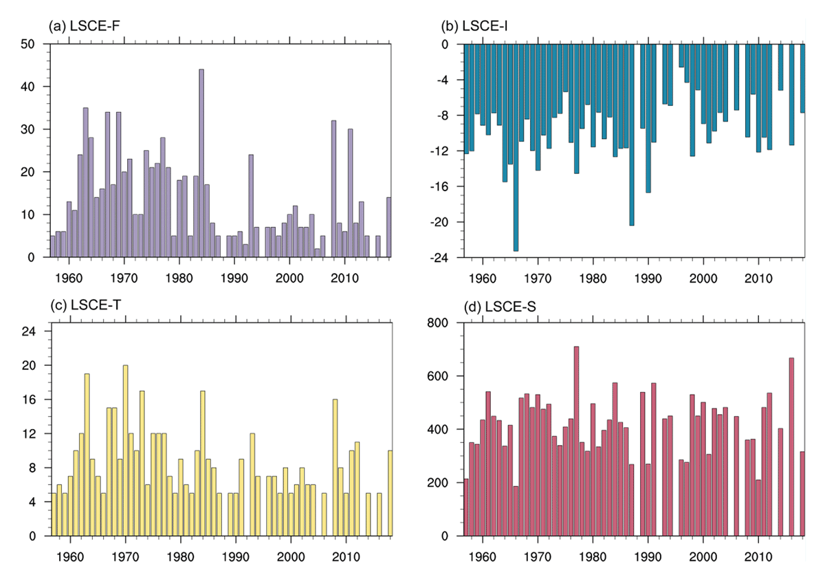
Figure 1a
Annual feature of winter time frequency of LSCE (LSCE-F, a), intensity of LSCE (LSCE-I, b), lasting-time of LSCE (LSCE-T, c), and scale of LSCE (LSCE-S, d) from 1958 to 2019.
In addition to the analysis of the frequency and intensity of LSCE, the scale and duration of the impact of LSCE across the whole country are also explored for every year. Here, the lasting time of LSCE for each year is defined as the LSCE-T (Figure 1c), and the number of total stations for one LSCE is regarded as the scale of LSCE (LSCE-S, Figure 1d). If the number of LSCE occurred more than once in one year, the average value of multiple affected stations is the number of LSCE occurrence stations per year. The lasting time of LSCE is based on the duration of more than 5 days in the filter conditions. Similarly, if there is more than one LSCE in a year, the average number of days of the multiple times is the number of days that the total LSCE last for each year. It can be seen from the evolution characteristics (Figure 1c) that there was also a certain amount of reduction of the LSCE-T around the 20th century and the overall change is not significant. However, in the late 20th century, the persistent impact of extreme cold events was significantly weaker than that before the 20th century. The duration of the former cold wave was basically about 6-8 days, while the latter could last up to more than 20 days. In comparison, when a cold event occurs, the affected area across the country (Figure 1d) has no decadal variation characteristics, but the annual variation characteristics are more obvious. Among them, the most affected areas were in 1977 and 2016, both reaching 700 stations, indicating that the cold events covered the whole country. There are more than 200 stations with a small impact area, indicating that the intensity of the cold wave is relatively weak and the impact area is greatly reduced.
After analyzing the characteristics of LSCE across the country, it can be seen that the annual variation of cold events especially the changes in intensity and scope are quite significant. Therefore, we then choose the typical strong and weak cases to see the differences thereof. Figure 2 shows the three strong cases of LSCE with the years are 2011, 2012 and 2016. For the cases (Figure 2), 2016 was the year with the strongest LSCE, followed by 2010 and 2012. It is worth noting that the areas most affected by LSCE are almost in northern China, and the temperature change in the south is relatively weak. Figure 3 displays the three weak cases of LSCE with the years are 1966, 1974 and 2010. As seen, the spatial distribution shows that the three events mainly covered the northeast region of China. In 1966, only the northeastern China is most affected by the LSCE. In addition, there are fewer stations are affected in the southwest of Tibet, because the stations are less than that in eastern regions of China. On the case, the temperature of the affected regions reached minus 14°C, and the temperature changes in other regions were not obvious. In 1974, the northeast China was affected by the cold event, of which Heilongjiang, Jilin and Inner Mongolia were mainly affected, reaching minus 12°C. The middle reaches of the Yangtze River in the south to Guizhou and Guangxi were also affected, with a drop in temperature of minus 4°C. During the cold event in 2010, the range from central Inner Mongolia to the Yellow River and the estuary of the lower reaches of the Yellow River was the most affected, with a drop in temperature of more than minus 12°C.
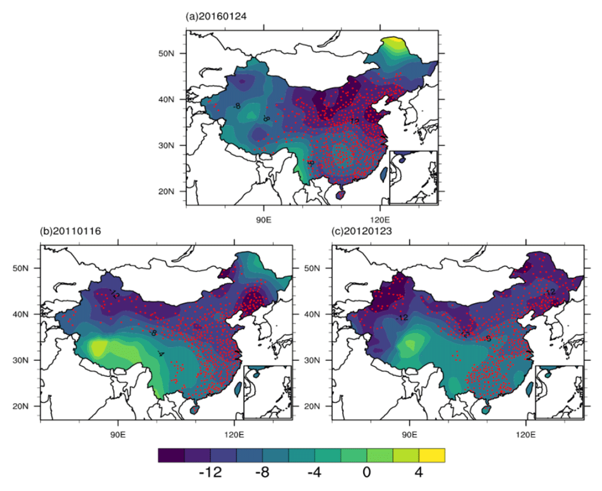
Figure 2
The spatial distribution of temperature anomalies (shaded, °C) and the affected stations (red points) in (a) 2016, (b) 2011, and (c) 2012.
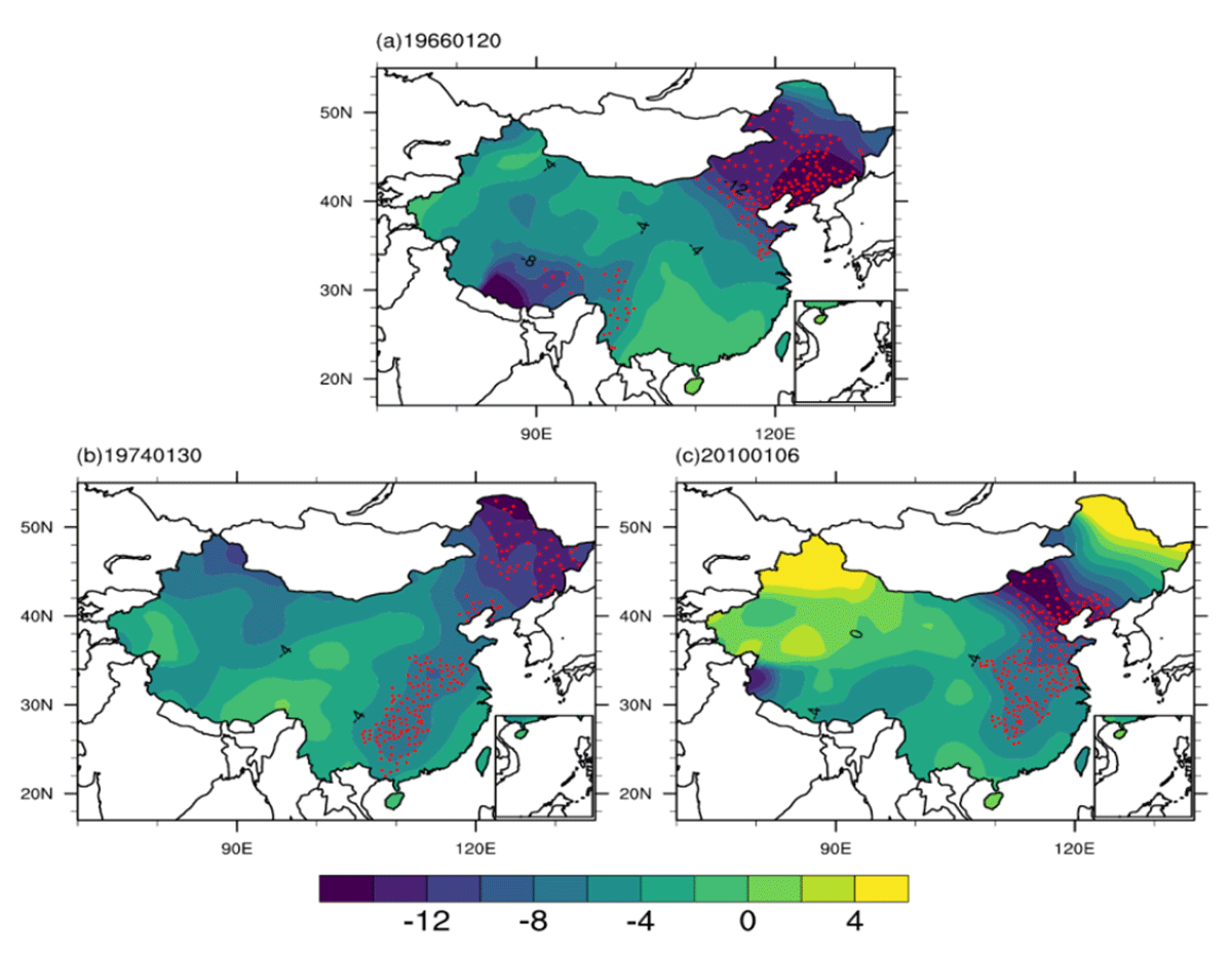
Figure 3
Same as Figure 2 but in (a) 1966, (b) 1974, and (c) 2010.
4. Different phases of MJO and their connection to the temperature in China
We use the method mentioned in section 2 to obtain the 8 phases of MJO as discussed in Wheeler et al. [34] that the convective activities over the tropics start from the Indian Ocean, migrate eastward to the Western Pacific Ocean. Here, we also give a snapshot on the changes of tropical activities from Phase 1 to Phase 8 in Figure 4. As shown, it can be clearly seen that the activities start from the eastern Africa coastline to western Indian Ocean regions (Phase 1, Figure 4a), and increase and transport eastward at the same time and with a maximum intensity in Phase 3. The activities migrate across the Indian Ocean, and the tropical oceanic and continental regions. When they come to the western Pacific Ocean (Phase 6), the intensity is decreased and further disappears in Phase 7 and Phase 8. These 8 phases exhibit the complete cycle of the tropical convective activities, which suggests the possible regional effects of tropics to the northward midlatitudes.
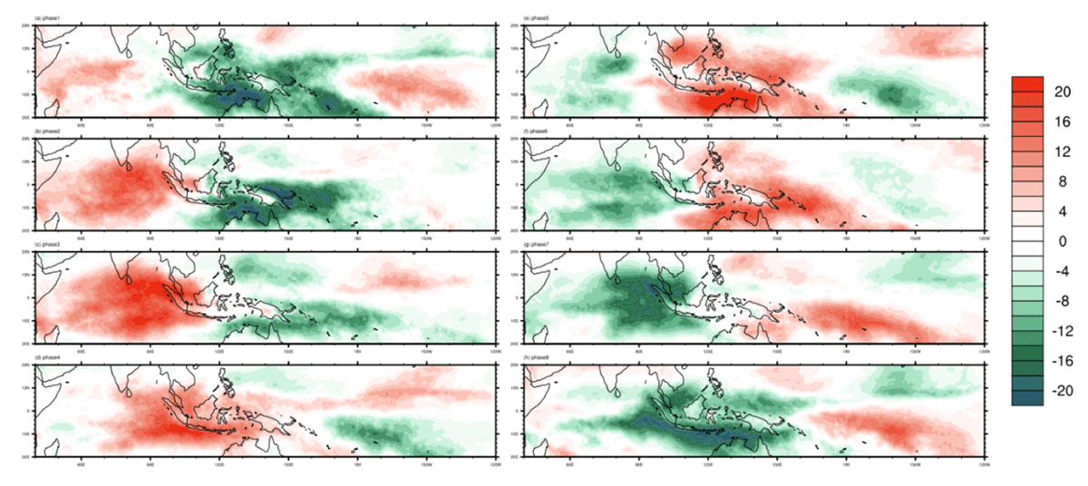
Figure 4
Spatial distribution of tropical OLR (shaded, W m-2) under the different phases of MJO. Here the values are multiply by –1 for clear recognition.
In addition, the effects of the different phases of MJO on the temperature are checked and illustrated in Figure 5. We can see the temperature anomalies show different features under different phases of MJO. Separately, the temperatures in Phase 1 and Phase 7 are increased all over the country, which is opposite to the features in Phase 2, Phase 3 and Phase 5. Besides, the temperatures in Phase 4 and Phase 7 show regional features and that in Phase 6 seems to have no changes. That is to say, the effects of MJO on the temperature in China are different in individual phase, which adds more difficulties for understanding the detailed features of temperature correlated to the MJO. One may say that although the effects are different, but if we could find which phase plays a dominated role in winter, the related abnormal temperatures are relatively easy to present. Thus, we inspect the occurrence of the 8 phases in an average winter for the period of 1979 to 2019 (Figure 6), and find that the occurrence of different phase shows only slight differences with minimum value of Phase 1 and maximum value of Phase 7. This indicates the challenges to outline the effects of the different phases of MJO on local temperatures in China.
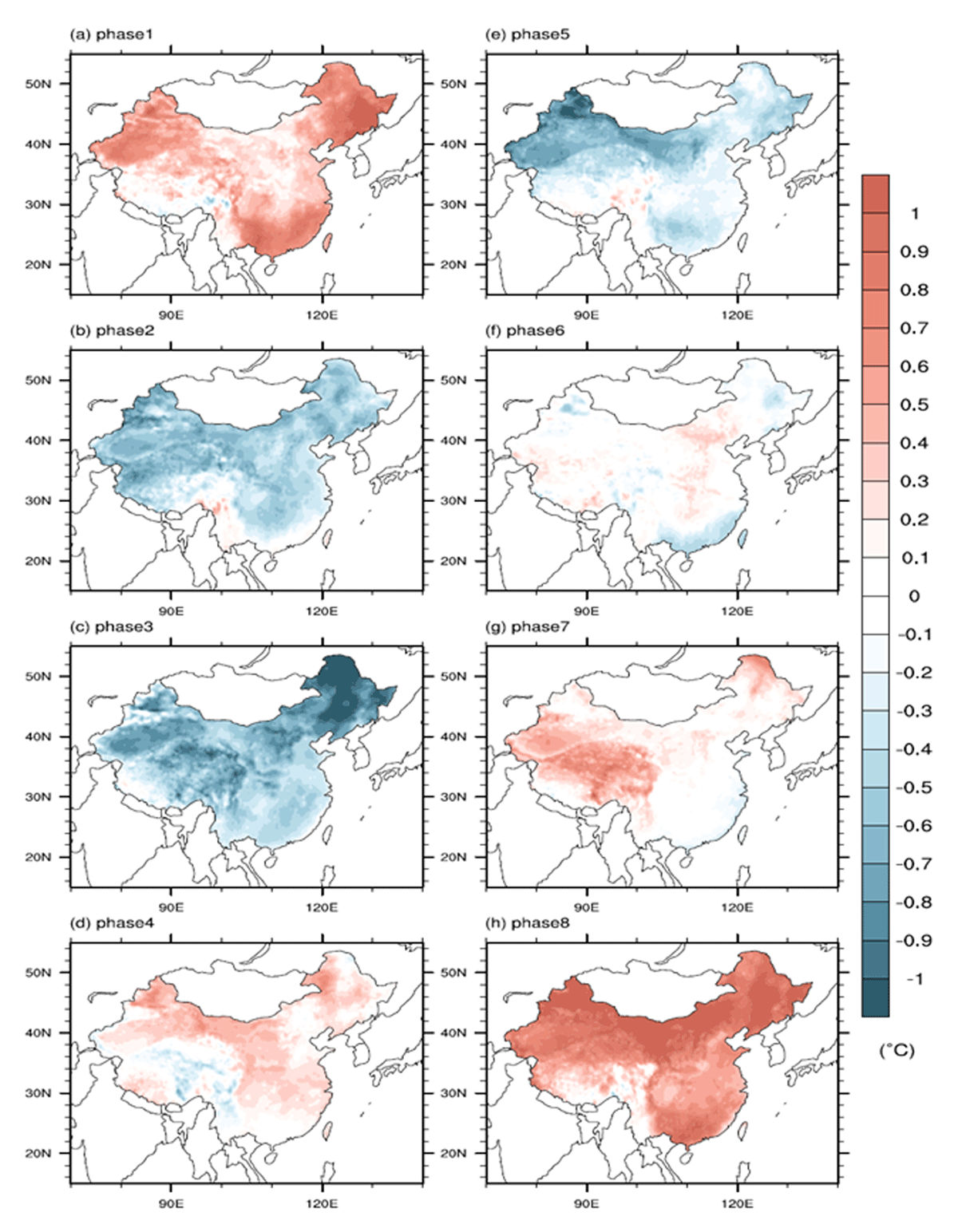
Figure 5
Spatial distribution of temperature anomalies for 8 phases separately.
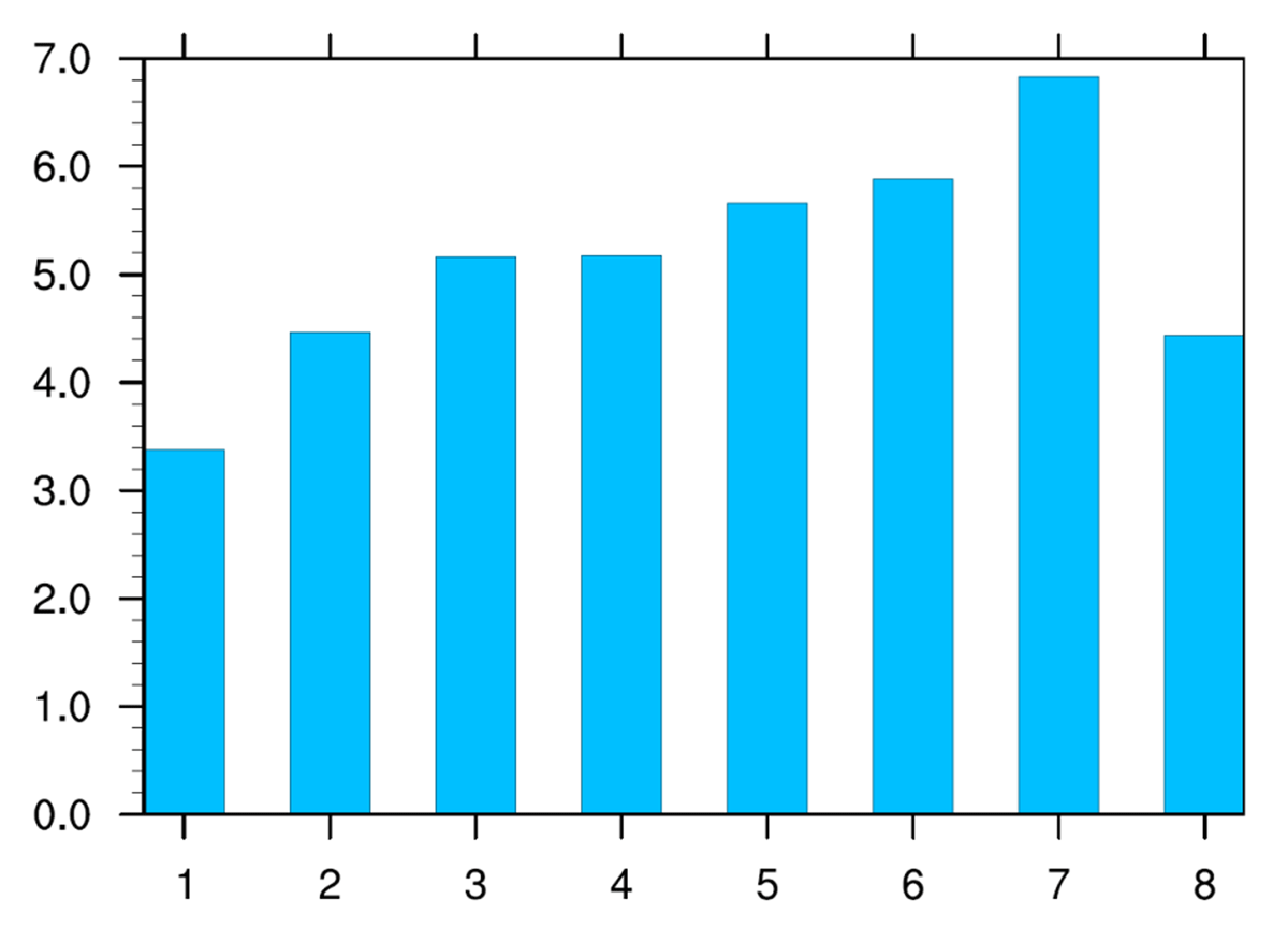
Figure 6
The average number of days for 8 phases in winter.
5. Spatiotemporal distributions of MJO and the corresponding features of cold events
Since it is hard to separate the individual effects of various phases of MJO on the temperature, here we attempt to examine the principal modes of MJO frequency (MJO-F) including all the phases. Figure 7 illustrates the first two modes of MJO-F and the corresponding time series on the annual variability. The first mode of empirical orthogonal decomposition for the MJO-F (EOF1) shows an opposite feature between Phases 1–3 and Phases 5–7 with the explanation of variance at 30.6%. This means the dominated phases of MJO in winter are positive ones of Phases 1–3 and negative ones of Phases 5–7, which indicates that the strong tropical convective activities over the Indian Ocean play a dominated contribution. As for EOF2, an opposite feature between Phases 4–5 and Phase 7 with the explanation of variance at 26%. This suggests strong tropical convective activities over the eastern Indian Ocean to tropical oceanic continents are important thereof. Besides, the time series (PC1 and PC2) of both EOFs show a significant annual variability and a large variance.
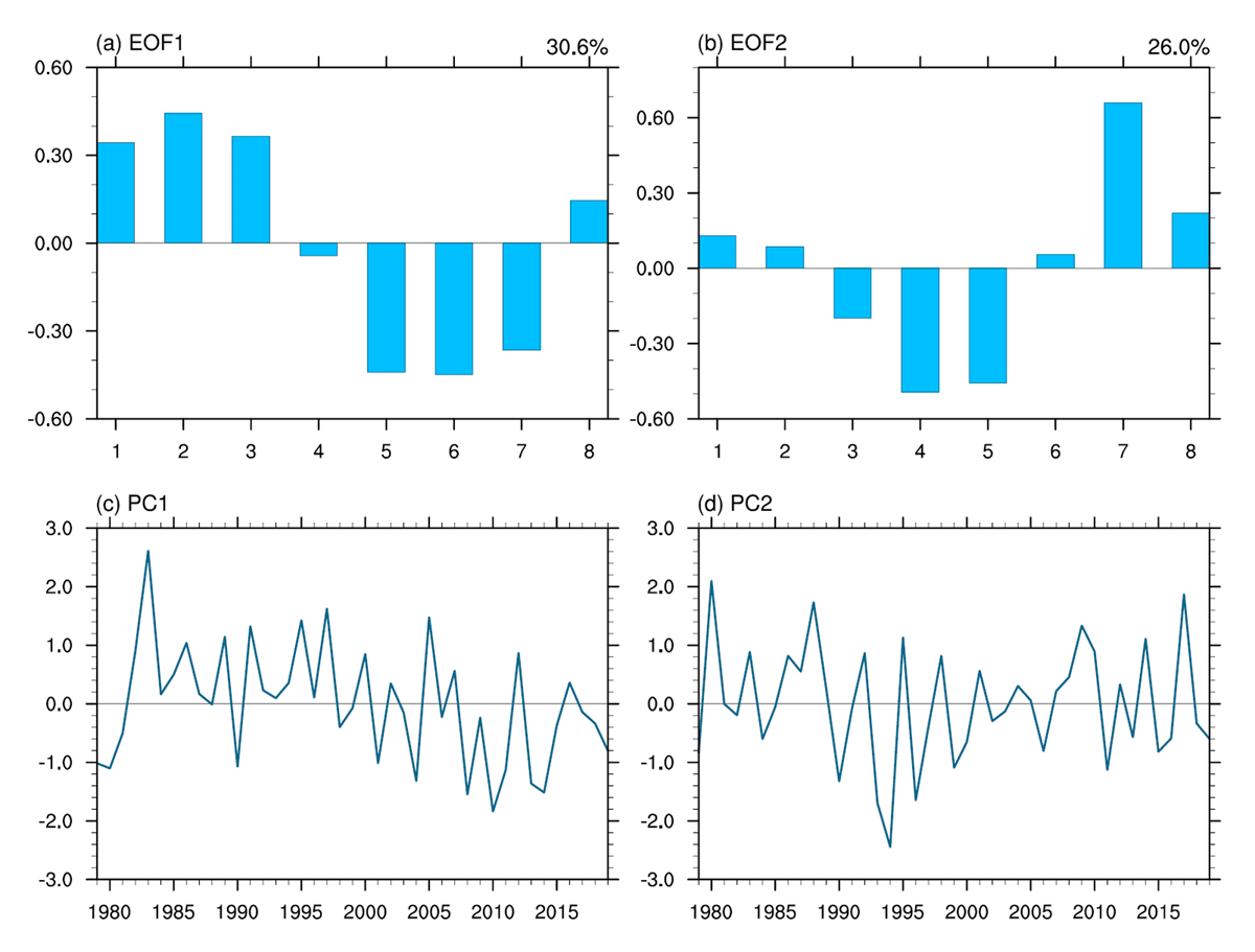
Figure 7
The first two EOFs (a and b) of MJO frequency in 1979–2019 winters, and the corresponding time series (c and d).
In order to check the features of temperature under the EOFs, we first define a threshold of ±1.5 according to the PCs in Figure 7, and then choose the years larger and lower than the threshold and clarify them into four cases that +PC1, –PC1, +PC2 and –PC2. Furthermore, we take all the LSCEs into consideration with a statistic analysis for each case. Last, a composite method is used to inspect the temperature anomalies for 4 cases separately. As shown (Figure 8), the temperature anomalies (500hPa) are different in the four cases associated with the LSCEs. For the case of +PC1, the temperatures are decreased in the whole country with the negative centers mainly covering the eastern China. For the case of –PC1, the temperatures are decreased without the southwestern China, and the negative anomalies over the northeastern China are stronger than the others. For the case of +PC2, the temperatures are significantly over the northeastern regions of China with stronger negative anomalies thereof. For the case of –PC2, the temperatures anomalies are relative weaker than the other cases, with the negative centers mainly over the northern China and southeastern regions over China. All the defined cases are the chosen LSCEs with respect to the positive and negative phases of MJO, and the results present the MJO-related LSCEs are somewhat stronger in specific regions. We also check the temperature anomalies between the MJO-related LSCEs and the LSCEs without consideration of MJO effects (Figure now shown), which further confirms the results obtained above.
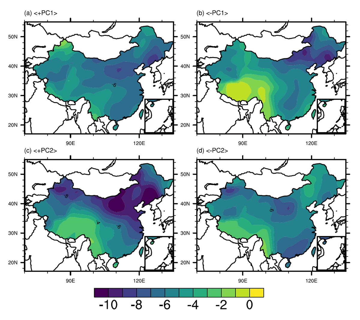
Figure 8
The spatial distribution of surface temperature anomaly at 500 hPa for the cases of (a) +PC1, (b) –PC1, (c) +PC2, and (d) –PC2, respectively.
6. Possible mechanism of the MJO phase variation to the cold extremes
Based on the analyses in last section, we can see the different wintertime configurations of MJO phases have significant effects on the regional LSCEs through altering the local temperature thereof. However, the possible mechanism still needs to be further investigated. Firstly, the corresponding atmospheric circulation anomalies under 4 cases are portrayed in Figure 9. For the case of +PC1 (Figure 9a), the positive and negative anomalies of geopotential height at 500 hPa (Z500) over East Asia imply the anticyclonic and cyclonic circulation there. The configuration of circulation anomalies especially the cyclonic circulations over the southeastern China to western Pacific regions are benefit to the persistence and development of cold spells. Thus, the negative anomalies over eastern China are shown in Figure 8a. Similarly, in Figure 8(b)–8(d), the cyclonic anomalies could be found over eastern Asia as well, corresponding to the negative temperature features displayed in Figure 7.
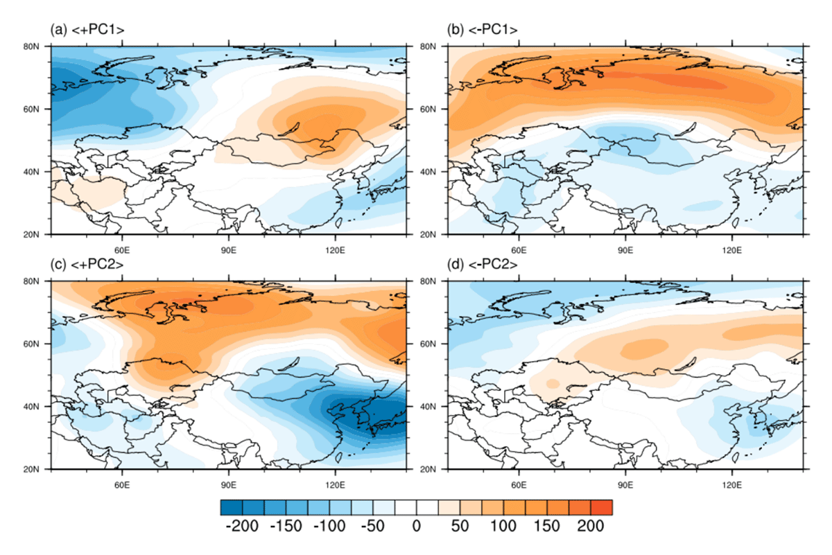
Figure 9
The spatial distribution of geopotential height anomaly at 500 hPa for the cases of (a) +PC1, (b) –PC1, (c) +PC2, and (d) –PC2, respectively.
In order to expound the thermodynamic processes controlling the variability of temperature associated with the MJO, we detect the temperature budget equation in Eq. (1), that the temperature anomaly tendency is affected by horizontal temperature advection, the adiabatic process associated with vertical motion and static stability, and diabatic heating processes:
, where, T is the temperature in each pressure level, t is the time, V is the horizontal velocity, 𝛻 is the Laplace operator, 𝜔 is vertical velocity, Q is atmospheric apparent heat source, and σ is the static stability (σ = RT/Cp – ∂T/∂P), where R is the gas constant, P is the pressure (Pa), and Cp is the specific heat at constant pressure. One meteorological factor could be separated into two parts, i.e. the mean state for a long period of time and the eddy state departure from the climatological feature. Thus, we decompose the variables in Eq. (1) into the mean and anomaly fields in Eq. 2 to understand the physical processes:
, where u and v are the zonal and meridional winds, respectively.
As in previous discussions (Qian et al., 2022; Xue and Zhang, 2017), the meridional transport of the mean state temperature gradient (–ν(∂T̅/∂y)) usually plays a key role in the temperature budget. Therefore, for simplicity, the second item of the right side of Eq.2 is calculated and shown in Figure 10. Compared to the surface temperature anomalies, it can be seen that for all the cases of four PCs, the temperature anomalies at 925 hPa are basically same as that in Figure 8. For the case of +PC1, the changes of temperature are located over eastern China, and the meridional winds show the southward anomalies, accompanied by the cold advection over the coastline regions to the western Pacific (Figure 10a). This means the cold air from higher latitudes transport to eastern Asia forming a cold temperature advection and negative temperature anomalies thereof. For the case of –PC1, besides the eastern regions of China, there still cold temperature advections transport from the Mongolia regions (Figure 10b), inducing the negative anomalies over the Inner Mongolia region (Figure 8b). For the case of +PC2 (Figure 10c), the southward wind and the accompanied cold advection are stronger than the others affecting mostly regions in China, which leads to the higher decrease of temperatures (shades in Figure 10c and Figure 8c). Last, for the case of –PC2 (Figure 10d), the cold advection and the southward wind are, opposite to that in +PC2 and weaker than others, resulting in the negative temperature anomalies mainly over the southeastern China.
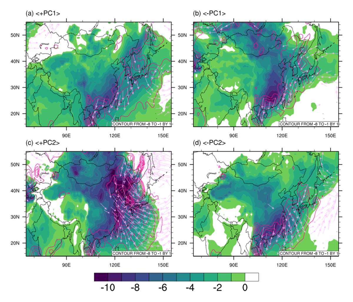
Figure 10
Same as Figure 9 but for the temperature anomalies (shades, °C), zonal wind (vectors, m/s), and horizontal advection of temperature (contours, °Cs–1).
7. Conclusions and discussion
This study investigates the effects of principal modes of MJO on the large scale cold events (LSCEs) in China. Firstly, the typical LSCEs have been identified and the corresponding characteristics of the LSCEs are also examined from diverse aspects. In addition, the different phases of MJO and the correlations to the local temperatures are checked. Since the individual effects of various phases of MJO on the temperature are hard to test, we examine the principal modes of MJO and further investigate the variations of modes on the local temperatures. Last, the possible contributions have been detected from the perspective of thermodynamics. The main results are listed as follows:
There are total 89 LSCEs from the wintertime period of 1959–2019 in China. The frequency, intensity, scale and lasting time of LSCEs (LSCE-F, LSCE-I, LSCE-S and LSCE-T) are examined from the time evolution features. The LSCE-F and LSCE-I have the decadal variability, that the values are much higher before 1990 than that after 1990. Besides, one can find the frequency and intensity both have a reduction of 60% and 45% respectively in the recent decades, which is possibly correlated to the background effects of global warming.
There was a certain amount of reduction of the LSCE-T around the 20th century and the overall change is not significant. However, in the late 20th century, the persistent impact of extreme cold events was significantly weaker than that of before the 20th century. In comparison, the affected area across the country (LSCE-S) has no decadal variation characteristics, but the annual variation characteristics are more obvious.
For the strong cases of LSCE, the areas most affected by LSCE are almost in northern China, and the temperature changes in the south are relatively weak. And for the weak cases of LSCE, the affected areas have the regional differences in difference cases, however, with a lesser temperature reduction than that in strong cases.
The effects of MJO on the temperature in China are different in individual phase, which adds more difficulties for understanding the detailed features of temperature correlated to the MJO. However, the first mode of MJO-F (EOF1) shows an opposite feature between Phases 1–3 and Phases 5–7 with the explanation of variance at 30.6%. This indicates the strong tropical convective activities over the Indian Ocean make a dominant contribution. As for EOF2, an opposite feature between Phases 4–5 and Phase 7 with the explanation of variance at 26%. This suggests strong tropical convective activities over the eastern Indian Ocean to tropical oceanic continents are important thereof. Besides, the time series (PC1 and PC2) of both EOFs show a significant annual variability and a large variance.
In order to check the temperature anomalies related to the MJO via the thermodynamic factors, the threshold of ±1.5 according to the PCs are used to clarify the difference events into four cases that +PC1, –PC1, +PC2 and –PC2. For the case of +PC1, the cold air from higher latitudes transport to eastern Asia forming a cold temperature advection and negative temperature anomalies thereof. For the case of –PC1, the cold temperature advection also transports from the Mongolia regions, inducing the negative anomalies over the Inner Mongolia region. For the case of +PC2, the southward wind and the accompanied cold advection are stronger than the others affecting mostly regions in China, which leads to the higher decrease of temperatures. For the case of –PC2, the cold advection and the southward wind are, opposite to that in +PC2 and weaker than others, resulting in the negative temperature anomalies mainly over the southeastern China. Meanwhile, with the transport of cold advections in all the chosen cases, the background cyclonic and anti-cyclonic circulation anomalies at higher altitudes are great beneficial to the maintenance and development of local cold extremes.
As discussed in this study, one can find the possible effects of the phase variations of MJO onto the regional temperatures related to the large scale cold events. Here we mainly focus on the principal mode of the frequency of MJO in wintertime, but there are also other factors like intensity need to be further inspected, which is beyond the scope of the current work. Besides, only the thermodynamic process is utilized for interpretation of the underlying mechanism between the MJO and the LSCEs in China, nevertheless the dynamic effects are necessary to be explored. Especially, the teleconnections between different latitudes are complex and arduous to be clearly elucidated. Here we give a prior attempt to investigate the changes of different phases of MJO and the preliminary discussion about the possible mechanism, more works mentioned above will be further inquired in the future works.
Acknowledgements
The authors thank the anonymous reviewer for many helpful comments, which greatly improved the article.
Funding Information
This research was funded by State Grid Technology Project (grant number 5216A0210040:5200-202123095A-0-0-00). In this study, the daily station records of temperature are taken from the China Meteorological Data Center (http://data.cma.cn/en/?r=data/detail&dataCode=A.0012.0001).
Competing Interests
The authors have no competing interests to declare.
Publisher’s Note
The funding information was altered from the original publication to reflect an update that hadn’t been acknowledged originally.