
1. Introduction
The global overturning is the largest-scale component of ocean circulation, ventilating deep water masses on decadal to millennial timescales (Talley 2013; Cessi 2019). The circulation connects water masses from different ocean basins, inducing a large-scale redistribution of heat, carbon and nutrients, making it central to Earth’s climate and biogeochemical cycles. The fundamental question of what drives the global overturning circulation – whether surface buoyancy forcing or mechanical forcing by winds and tides – has been a contentious issue in the oceanographic community starting as early as the 1870s (Mills 2009), and still has not been satisfactorily settled to date. Nevertheless, identifying the important drivers at different time scales is crucial to understand the ocean response to climate changes.
The overturning circulation is obtained from zonally integrating the meridional velocity, yielding two cells in the latitude-depth plane. The global overturning is composed of two main cells, an upper cell which reflects flow primarily in the Atlantic basin and is associated with North Atlantic Deep Water (NADW), and a lower cell concentrated in the Indo-Pacific basins associated with Antarctic Bottom Water (AABW) (Talley 2013). The cells are separated by a region of heightened stratification, between about 1000 and 2000 m depth, roughly coincident with the 5°C isotherm (Figure 1). The mid-depth stratification reflects the fact that the AABW does not upwell to the surface, but is confined to the deepest levels.
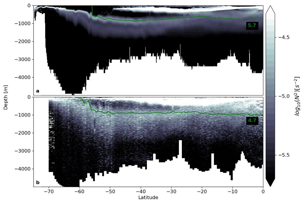
Figure 1
Stratification in a realistic model and observations. (a) Model output of stratification, shown as log10(|N2|), from a realistic eddying ice-ocean model (Kiss et al. 2020) at a longitude of 110°W, shown for the (Austral) winter month of September 2015. The green line is the isotherm T = 5.7°C. (b) Ship-based observations of stratification, shown as log10(|N2|), for WOCE transect P18 (between longitudes 110°W and 100°W) from a R/V Ronald H. Brown cruise in November 2016–February 2017. The green line is the isotherm T = 4.7°C.
A central and long-standing question is what drives these cells. Early thinking was influenced by Stommel (1958) and Stommel and Arons (1959), who examined the abyssal circulation driven by sources of dense water in specified locations in the higher latitudes. This work led to the prediction of deep western boundary currents, which hitherto had not been observed. Critically, it was assumed that upwelling, needed to close the circulation, is uniform in the ocean interior. Subsequent work sought to explain the observed thermocline structure in terms of a one-dimensional balance between the constant upwelling and diffusion in the vertical (Munk 1966). This resulted in a diffusivity estimate of order of 10–4 m2/s. However, subsequent measurements revealed the diffusivity in the ocean interior is at least an order of magnitude less (Gargett 1984; Ledwell et al. 1993). Thus a hunt for the “missing mixing” began, leading to a better understanding of the distribution of ocean interior dissipation, with mixing hotspots found over rough topography (Polzin et al. 1997).
Weak mixing would favor regions of strong stratification in the interior, as “internal boundary layers” (Salmon 1990). Further, the overturning should be close to adiabatic in the interior. This led to the suggestion that overturning in the upper cell was linked to wind-driven Ekman transport from the Southern Ocean (Toggweiler and Samuels 1995, 1998; Marshall and Speer 2012). The zonally-integrated Ekman transport is of order 30 Sv (Talley et al. 2011), comparable to the maximum overturning in the upper cell. The zonal winds steepen the isopycnals, which spawn mesoscale eddies whose fluxes flatten the density surfaces via baroclinic instability (Gent et al. 1995). Southward fluxes by these eddies are thought to partially compensate the northward Ekman flux. The residual transport is posited to link with the northern overturning (Gnanadesikan 1999; Marshall and Radko 2003; Radko 2005; Henning and Vallis 2005; Wolfe and Cessi 2010; Nikurashin and Vallis 2012; Marshall and Speer 2012; Johnson et al. 2019; Cessi 2019).
The deep cell on the otherhand is thought to be driven by mixing (e.g. Cessi 2019). The mixing derives primarily from wind- and tidally-driven motion (Munk and Wunsch 1998; Wunsch and Ferrari 2004). Thus both cells are linked to mechanical forcing, either directly (wind-driven upwelling in the Southern Ocean) or indirectly (wind- and internal tide-induced mixing in the interior).
Buoyancy forcing is believed to be less important. This follows from laboratory experiments conducted in the early 1900s, which showed that a circulation driven solely by surface buoyancy forcing would collapse to a thin layer at the surface with vanishing interior mixing (Sandström 1908, 1916), an inference later known as “Sandström’s theorem” (Defant 1961). Sandström’s view was challenged by Jeffreys (1926) who questioned the relevance of weak mixing to a turbulent ocean. But a subsequent study (Paparella and Young 2002) demonstrated that a purely buoyancy-driven flow would cease to be turbulent in the limit of a vanishing vertical diffusivity. The applicability of this result to the ocean has also been questioned (Scotti and White 2011; Gayen et al. 2014), but the notion that buoyancy forcing alone would only produce a weak, surface-trapped flow persists (Munk and Wunsch 1998; Wunsch 2000).
In other laboratory studies however (Rossby 1965; Park and Whitehead 1999; Mullarney et al. 2004), and in models of varying complexity (Bryan 1987; de Verdière 1988; Huck et al. 1999; Scotti and White 2011; Gayen et al. 2013; 2014; Pedlosky 1969; Salmon 1986; LaCasce 2004; Hughes and Griffiths 2006; Gjermundsen and LaCasce 2017; Gjermundsen et al. 2018), buoyancy forcing has been found to drive a deep-reaching overturning circulation. The circulation has become known as “horizontal convection” (Stern 1975; Hughes and Griffiths 2008) or “rotating horizontal convection” when planetary rotation becomes important (Barkan et al. 2013; Gayen and Griffiths 2022).
In a closed mono-hemispheric basin, rotating horizontal convection produces horizontal gyres with a western boundary current like the Gulf Stream, and dense water formation at high latitudes, as observed in the North Atlantic basin (Hogg and Gayen 2020; Gayen and Griffiths 2022). However, the buoyancy-driven flows in closed basins do not lead to the vertical penetration of the thermal forcing unless unrealistically large vertical diffusivities are employed. Nor can it produce the deep stratification which is a signature of the two-cell overturning circulation. However, deep stratification can be achieved in a re-entrant channel. This was demonstrated by Barkan et al. (2013) and later by Sohail et al. (2019) using turbulence-resolving direct numerical simulations of flow driven by a specified surface density profile. A baroclinically unstable zonal flow develops, similar to the Antarctic Circumpolar Current. In these experiments, eddies are responsible for most of the vertical and lateral buoyancy fluxes, rather than vertical diffusion alone. This demands large merdional buoyancy gradients, resulting in deep stratification.
The results of Barkan et al. (2013) raise the question – can the presence of a re-entrant channel allow a purely buoyancy-generated flow being to generate mid-depth stratification and a deep-reaching, two-cell, overturning circulation? Answering this question is the central goal of the present work.
Since the opening of the Tasman Gateway and Drake Passage some 30 million years ago, the Southern Ocean has been zonally unblocked, creating a re-entrant channel (e.g. Scher and Martin (2006); Sauermilch et al. (2021)). In contrast, the Pacific, Indian and Atlantic ocean basins are zonally blocked to the north of Drake Passage. The modern global ocean is therefore a combination of closed basins and a re-entrant channel. Thus, a suitable idealized basin geometry to represent the global ocean has a re-entrant channel in the south and lateral boundaries to the north (Gill and Bryan 1971; Cox 1989; Toggweiler and Samuels 1998; Wolfe and Cessi 2010, 2011; Nikurashin and Vallis 2012; Shakespeare and Hogg 2012).
To this end, we will use an eddying numerical ocean model with this basin geometry to understand the three-dimensional circulation resulting from surface buoyancy forcing alone. We examine, in order, simulations using (a) a fully closed basin, (b) a basin which is re-entrant over its entire latitude range, and (c) a single-hemisphere basin combining zonal boundaries with a southern re-entrant channel. We then use these building blocks to describe the three-dimensional overturning circulation generated by surface buoyancy forcing for the most realistic domain, with (d) a southern re-entrant channel connected to an elongated basin that extends to the northern high latitudes. To weigh the limitations of primitive equation models, such as numerical diffusion and the parameterisation of convection, we compare our results to laboratory experiments and direct numerical simulations wherever possible. Due to work on rotating horizontal convection currently existing only for fully blocked domains and a re-entrant channel, but not a combination of the two, the comparisons will be limited to these domains.
2. Model description
We employ the Massachusetts Institute of Technology general circulation model (MITgcm, Marshall et al. (1997)) in an idealised domain in spherical coordinates. This takes into account the full variation of the Coriolis parameter, f = 2Ωsin(θ), where θ is the latitude. The model configuration is based on that of Munday et al. (2013), with the main difference being that we restrict attention to thermal forcing.
The model domain is 20° in longitude, and extends from 60°S to 60°N. Using a narrow sector allows for running multiple simulations for thousands of years in a computationally efficient manner. The latitudinal extent allows for a full interhemispheric overturning circulation with convection both in the south and the north, and allows the stratification and overturning circulation to evolve together dynamically. The horizontal model grid spacing is 1/6° in the zonal direction, whereas the grid spacing in meridional direction is scaled by the cosine of latitude, making the grid boxes approximately square. For the flow in the realistic domain, the model resolves the internal deformation radius over most of the domain, specifically from 50°S to the northern boundary. The domain has a flat bottom with a depth of 5000 m, discretised by 42 unevenly spaced levels with a thickness of 10 m at the surface, increasing to 250 m at depth. We use a linear equation of state, with a thermal expansion coefficient of α = 2 × 10⁻⁴K–1, a 7th order advection scheme, and a Leith viscosity parameterisation. The explicit vertical diffusivity in the reference case is set to κ = 10–6m2s–1 which falls between molecular values (~10–7m2s–1) and observed values (~10–5m2s–1). We employ no parameterisation for mesoscale eddies, having an eddy-permitting horizontal resolution, and no mixed-layer turbulence closure parameterisation, as there is no applied surface wind mixing.
Within the top-most 10 m of the water column (i.e. the top-most grid cell of the model) we restore to an idealised profile of potential temperature (henceforth temperature) with cold water at the northern and southern boundaries, and warm water at the equator (Figure 3(a)). The functional form of this temperature profile is given by
where TS is the temperature at the southern boundary, ΔT is the temperature difference between the southern boundary and the equator, TN is the temperature at the northern boundary, and θ is the latitude. The restoring timescale is 10 days. For our reference experiment we use TS = 0°C, ΔT = 30°C, and TN = 5°C.
We use four different domains to highlight the role of a circumpolar channel on the buoyancy-driven overturning (Figure 2(a–d)). Three of these, shown in Figure 2(a,b,d), cover both hemispheres, from 60°S to 60°N, with the remaining domain being limited to the Southern Hemisphere (Figure 2(c)). The first domain is the blocked domain (Figure 2(a)) with walls along its entire meridional extent, similar to the experimental configurations of many laboratory experiments and direct numerical simulations of (rotating) horizontal convection. In the second domain, the re-entrant domain (Figure 2(b)), we now remove the walls bounding the domain to the east and west, along its full meridional extent. The two remaining domains, the equator domain (Figure 2(c)) and the realistic domain (Figure 2(d)), are a combination of the first two, with a re-entrant channel which extends 20° in latitude in the south, and a blocked region to the north of the channel. The equator domain is limited to the southern hemisphere, while the realistic domain covers the full latitude range. All simulations are run for 4000 years, with mean values being a mean over the last 20 years. The overturning circulation shown is calculated as a residual overturning on density surfaces, and then re-mapped onto depth coordinates.
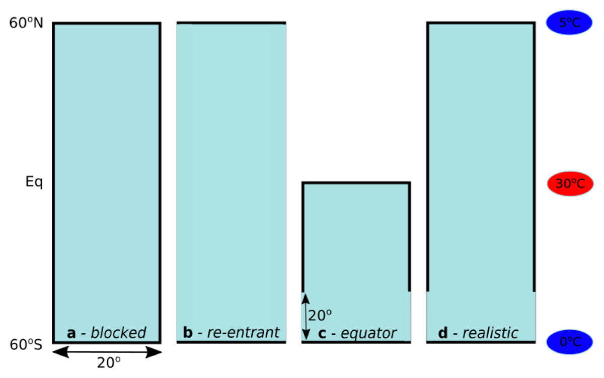
Figure 2
Model domains. (a) Model domains used for the experiments are (a) blocked, (b) re-entrant, (c) equator, and (d) realistic. All domains extend 20° in longitude, and from 60°S to 60°N in latitude, apart from the equator domain which is limited to the southern hemisphere. The re-entrant channel in the (c) equator and (d) realistic domain extends 20° in latitude. Black lines are solid boundaries, whereas blue boundaries are re-entrant, that is, fluid which leaves the domain in the east (west) enters the domain in the west (east). The temperature at the equator is restored to 30°C, the southern end of the domain to 0°C, and the northern end of the domain to 5°C.
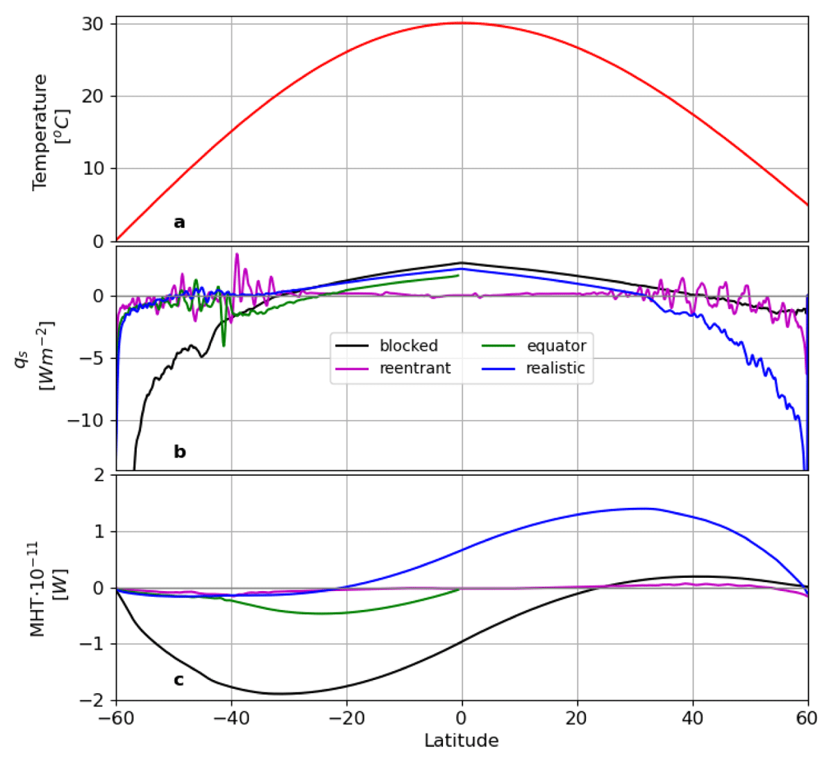
Figure 3
Surface forcing and meridional heat transport. (a) Sea-surface temperature restoring profile, (b) resulting temperature fluxes (qs), and (c) meridional heat transport (MHT) for the blocked (black), re-entrant (magenta), equator (green), and realistic (blue) domains.
3. Results
a. Circulation in a blocked domain
To illustrate the domain dependence of rotating horizontal convection, we begin with the simple blocked case (Figure 2(a)), as used in many previous laboratory and direct numerical simulations. The restoring surface temperature profile (Figure 3(a)) results in buoyancy (heat) fluxes (Figure 3(b), black line) that are stabilizing (due to heating) at low latitudes and destabilizing (due to cooling) at high latitudes.
Also shown in Figure (3c) is the meridional heat transport, obtained by integrating the surface fluxes,
where qs is the downward temperature flux at the ocean surface, Lw is the width of the domain, and Re the Earth’s radius. The transport is of order 1011 W, which is roughly four orders of magnitude weaker than observed (Trenberth and Solomon 1994; Jayne and Marotzke 2002); the smaller value here is due primarily to having a narrower basin and the low values of vertical diffusion which we use throughout the water column. In the blocked case, the transport is asymmetric, with the transport to the south below roughly 20°N. This is due to the asymmetry in the surface forcing, which yields colder conditions at the southern boundary. The heat transport is carried primarily in the western boundary currents, discussed hereafter.
A stratified thermal boundary layer develops at the surface due to the stabilizing buoyancy flux at low latitudes. Consistent with this surface-intensified stratification, we also find the overturning circulation to be confined to the upper parts of the water column (Figure 4(c)). The main difference with most laboratory and direct numerical simulations of rotating horizontal convection in a blocked domain is that here we prescribe a surface temperature profile over the entire latitude range. This leads to two regions of destabilizing buoyancy flux (cooling), one at the southern (“Antarctic”) boundary and one at the northern (“Arctic”) boundary. Since the temperature at the southern boundary is substantially lower (by 5°C), the entire overturning circulation is biased towards the southern boundary. This is consistent with the laboratory study of Coman et al. (2010), which showed that in the case of two regions of destabilizing buoyancy flux, if the heat input between these two regions differs by more than 10%, the interior stratification is set by the stronger plume.
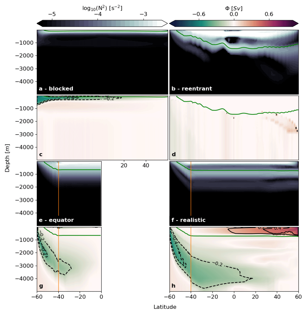
Figure 4
Stratification and overturning circulation; sensitivity to domain geometry. Vertical sections of zonal and temporal mean values of (a,b,e,f) the stratification, N2, shown as log10(|N2|), and (c,d,g,h) the overturning circulation (also shown as black contour lines), Φ, for the (a,c) blocked, (b,d) re-entrant, (e,g) equator, and (f,h) realistic domain. The orange lines mark the northern extent of the circumpolar channel, and the green lines mark the 5°C isotherm.
In the horizontal, surface buoyancy forcing produces a vertically-sheared zonal flow, as noted above and described in previous studies (de Verdière 1988; Gjermundsen and LaCasce 2017). The zonal flow is supplied by a poleward flowing western boundary current (Figure 5(b)), and deepwater formation occurs largely in the southeastern corner where the southern boundary supports a pressure gradient (Marotzke and Scott 1999), feeding an equatorward-flowing deep western boundary current. When the southward western boundary current passes from the region of stabilizing buoyancy flux to the region of destabilizing buoyancy flux (Figure 5(d)), stronger convection appears at the boundary. This convection penetrates deeper into the stable stratification below until this stratification is fully removed, and a full-depth convective plume occurs at the headwall, as seen in traditional horizontal convection (Gayen et al. 2014).
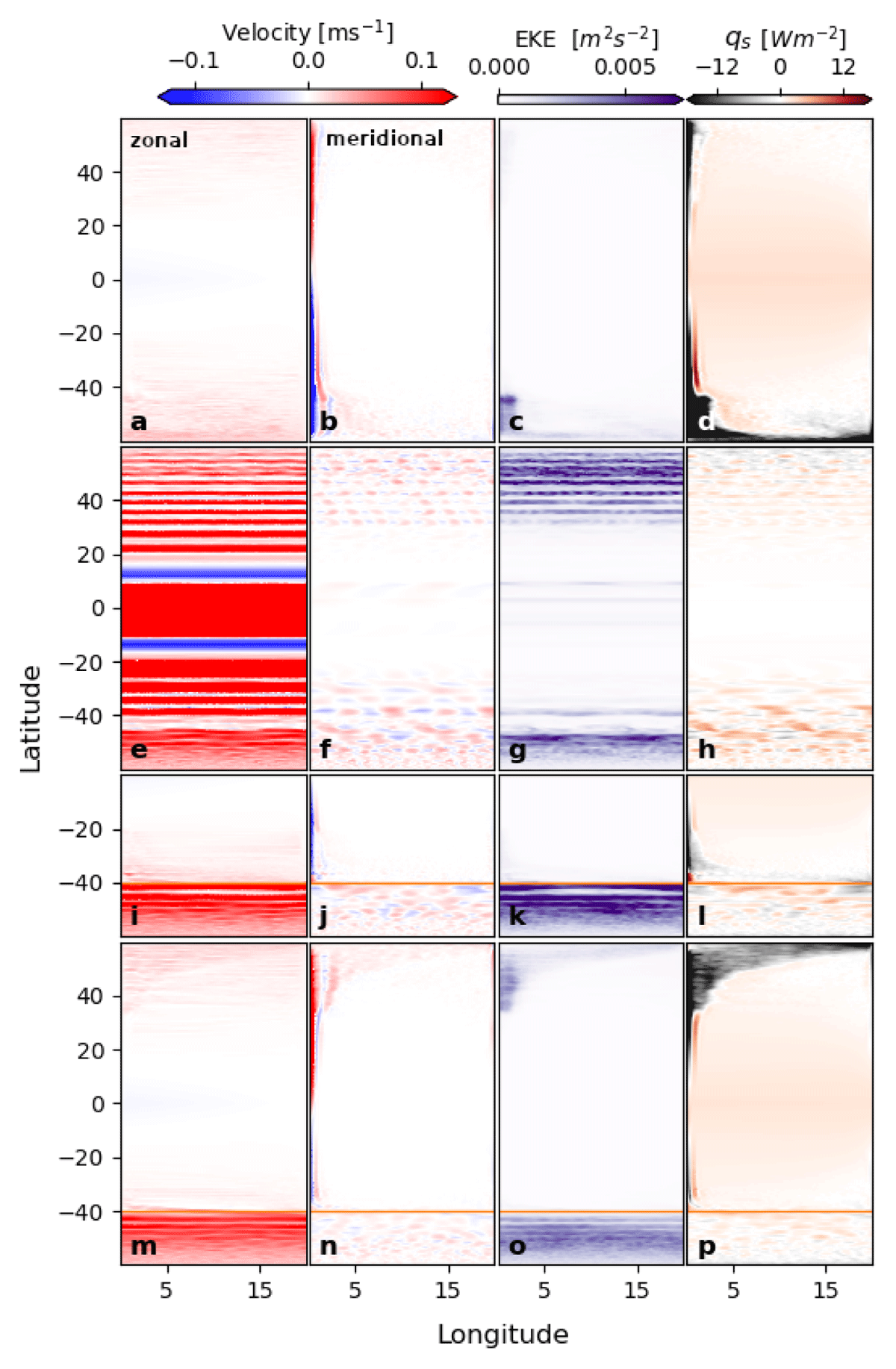
Figure 5
Horizontal circulation. Mean surface values of the (a,e,i,m) zonal velocity (U), (b,f,j,n) meridional velocity (V), (c,g,k,o) eddy kinetic energy (EKE), and (d,h,l,p) surface temperature fluxes (qs) for the experiment in (a,b,c,d) the blocked domain, (e,f,g,h) the re-entrant domain, the (i,j,k,l) the equator domain, and the (m,n,o,p) the realistic domain. The orange lines mark the northern extent of the circumpolar channel.
The transition from stabilizing buoyancy flux to the region of destabilizing buoyancy flux is also associated with a region of maximum baroclinic eddy activity (shown as regions of high eddy kinetic energy (EKE) in Figure 5(c)), in agreement with direct numerical simulations (Vreugdenhil et al. 2017), and is in general stronger in regions of destabilizing buoyancy flux and hence regions of convection. A strong velocity divergence along the western boundary currents (Figure 5(b)) is associated with a enhanced surface heat fluxes (Figure 5(d)). This is consistent with large vertical velocities in idealized modelling studies (Pedlosky and Spall 2005), ocean synthesis products and eddying ocean models (Liao et al. 2022), and a divergence in eddy heat fluxes observed from satellite altimetry (Müller and Melnichenko 2021). The idea of diverging heat fluxes matching the sense of the circulation is also consistent with a framework in which a volumetric census of density classes, and the fluxes between them, allows the residual circulation to be derived in a physically consistent manner (Walin 1982).
In summary, surface buoyancy forcing in the blocked domain leads to a shallow horizontal circulation with strong western boundary currents. There are convective plumes at the headwall and an associated overturning circulation. This circulation is in agreement with buoyancy-forced gyres simulated using both direct numerical simulations and eddying ocean models (Vreugdenhil et al. 2019; Hogg and Gayen 2020). Similar to results from coarse-resolution ocean models (Toggweiler and Samuels 1998), the western boundary currents are very efficient at transporting heat. Full-depth convection produces a uniformly cold abyssal ocean, forcing the vertical temperature gradients to the surface. In agreement with previous work, surface buoyancy forcing applied to a blocked basin can not generate the mid-depth stratification and overturning observed in the real ocean (Figure 4(a) vs. Figure 1). In addition, the thermal boundary layer is very shallow, a few hundred of metres thick, as expected for weak vertical diffusion.
b. Circulation in a fully re-entrant domain
We now remove the meridional walls in the blocked domain, creating a fully re-entrant domain with the flow now being unimpeded in the zonal direction (Figure 2(b)). Due to the absence of any wall in the zonal direction, no east-west pressure gradient can exist, and hence no western boundary current can be supported. The result is that the meridional heat transport, which is poleward in both hemispheres, is strikingly weaker than in the blocked domain (Figure 3c, magenta curve).
In the re-entrant case, the meridional heat transport is carried by baroclinic eddies. These are associated with strong zonal flows in the form of jets (Figure 5(e)). As in the blocked domain, the eddies are stronger in regions of destabilizing buoyancy flux (Figure 5(g)). The eddy transport is facilitated by steep isotherms (green line in Figure 4(b)). As such, the stratification extends to much greater depths than with the blocked domain (Figure 4(a) vs. (b)). This is also evident from the differences in depths of the 5°C isotherms (green lines in Figure 4(a) vs. (b)). This case closely resembles that studied by Barkan et al. (2013), who also found deep stratification with a re-entrant geometry. But as noted, the total heat transport is much weaker than with lateral boundaries present, consistent with a very weak overturning circulation (Figure 4(d)).
c. Circulation in a single-hemisphere domain with a southern re-entrant channel
We now consider the equator domain, a southern domain extending to the equator, combining blocked latitudes north of 40°S and re-entrant channel in the south (Figure 2(c)). The equator domain has a destabilizing buoyancy flux (cooling) in the south only (Figure 3(b)).
In the re-entrant channel of the equator domain, the circulation is similar to that in the re-entrant domain. The isotherms in both domains slope from the surface in the south to about 1000 m depth at 40°S, as evident from the 5°C isotherm (compare Figure 4(b) and 4(e), green line). In both cases, the sloping isotherms are associated with eddies (Figure 5(g,k)) and strong zonal jets (Figure 5(e,i)). As observed in the re-entrant domain, eddy fluxes in the re-entrant channel lead to deep stratification (Figure 4(e)). This deep stratification is generated through the projection of the cross-channel surface temperature gradient into the vertical by eddy fluxes along the sloping isotherms of the channel. The blocked part of the domain displays a western boundary current extending from the equator to the northern edge of the channel (Figure 5(b,j)). The thermal boundary layer depth is constant from the edge of the channel to the equator wall, and is significantly deeper than in the blocked domain (4 a). Thus the thicker thermal boundary layer is a direct result of eddy fluxes in the re-entrant part of the domain. This thick thermal boundary layer, together with the poleward heat transport by the western boundary current, allows for the generation of a strong lower overturning cell with its transport being dominated by eddies (Figure 4(g)), consistent with direct numerical simulations (Barkan et al. 2013; Sohail et al. 2019). The western boundary current permits a stronger meridional heat transport than in the re-entrant portion of the domain (Figure 3c, green curve), and hence a stronger lower overturning cell (Figure 4(g)).
d. Two-way interaction between northern and southern sinking regions
We now consider the realistic domain, which is similar to the equator domain in that it combines a re-entrant channel south of 40°S with a blocked basin to the north, but with the difference that it now extends to 60°N. With the extension northward to 60°N, the present set-up includes a second region of destabilizing buoyancy flux near the northern boundary (Figure 3(b)), magenta line). The inclusion of this second region of destabilizing buoyancy flux leads to the enhanced stratification observed over the top 2000 m of the water column in the equator domain (Figure 4(e)) to split into a thin layer of surface-intensified stratification, as observed in the blocked domain (Figure 4(a)), and two thin layers of enhanced mid-depth stratification (a stronger layer at a depth of about 1000 m, and a weaker layer at a depth of about 2000 m) (Figure 4(f)). This therefore results in two thermal boundary layers, and, due to the presence of both the presence of these thermal boundary layers and the western boundary currents which efficiently transport heat towards the convection regions, two major overturning cells (Figure 4(h)). A clockwise upper overturning cell is associated with the destabilizing buoyancy flux at the northern boundary. Meanwhile, a counterclockwise lower overturning cell is associated with the destabilizing buoyancy flux at the southern boundary. In addition, a weak re-circulation region exists between the two thermal boundary layers at mid-depths.
As demonstrated using the equator domain, the steeply sloping isopycnals result in the horizontal temperature gradient at the surface, ranging from 0°C at the southern boundary to about 12°C at the northern edge of the channel, to be mapped to a vertical distribution at the northern edge. This stratification is maintained through the entire blocked part of the domain, with little vertical variation. This deep stratification then sets the depth to which fluid cooled to 5°C can convect at the northern headwall. Since convection destroys stratification, the thick thermal boundary layer of the equator domain now collapses into a thin thermal boundary layer at the base of the northern convective plume. This thermal boundary layer, or mid-depth stratification, is therefore a result of the two-way interaction between southern and northern sinking region (Wolfe and Cessi 2010, 2011), with the channel dynamics – a balance between the vertical plume against the headwall and eddies – providing the stratification for the northern convective region to work against. This two-way interaction therefore leads to two thermal boundary layers, one at the surface and one at mid-depth, and hence two overturning cells. The resulting lower overturning circulation is stronger than in the equator domain, likely due to an increased heat transport to mid-depth by the upper overturning cell.
The process of generating a mid-depth stratification explained above also depends on the surface temperature at the northern boundary being warmer than at the southern boundary. As long as this requirement is fulfilled, an increase in surface temperature at the northern boundary, relative to that in the south, leads to a shallower and stronger mid-depth stratification. A decrease in surface temperature at the northern boundary leads to a deeper and weaker mid-depth stratification. This is consistent with direct numerical simulations that suggest that the overturning circulation is sensitive to interhemispheric differences in temperature forcing (Coman et al. 2006). If the northern boundary temperature is the same, or lower, than the southern boundary temperature, an abrupt change occurs and the mid-depth stratification disappears (Figure 7(a)). With the disappearance of the mid-depth stratification, both the lower overturning cell (Figure 6(d)) and the transport of the circumpolar current (Figure 6(a)) vanish since they both rely on heat supply across this interface. The existence of both the circumpolar current and the lower overturning cell therefore depends on the fluid sinking at the northern boundary being warmer than the fluid sinking at the southern boundary, hence being able to generate a vertical temperature gradient associated with the thermal boundary layer.
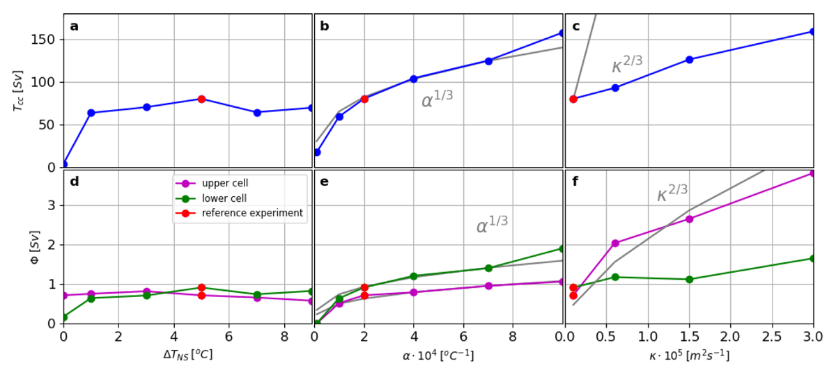
Figure 6
Circumpolar current transport and overturning strength. The circumpolar current transport, Tcc is shown as a function of (a) the north-south temperature difference, ΔTNS, (b) the thermal expansion coefficient, α, and (c) the vertical diffusivity, κ. The strength of the overturning circulation, Φ, is shown for both the upper (magenta) and lower (green) cell as a function of (d) the north-south temperature difference, ΔTNS, (e) the thermal expansion coefficient, α, and (f) the vertical diffusivity, κ. The red dots show values for the reference experiment. Grey lines show scaling arguments.
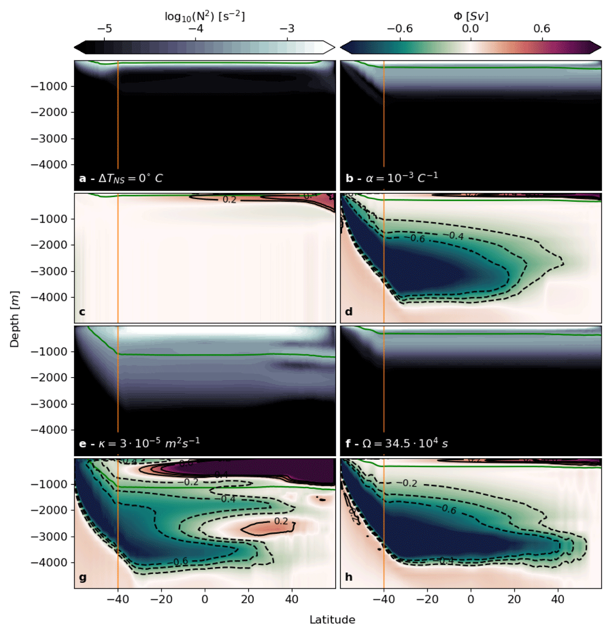
Figure 7
Stratification and overturning circulation; parameter sensitivity. Vertical sections of zonal and temporal mean values of (a,b,e,f) the stratification, N2, shown as log10(|N2|), and (c,d,g,h) the overturning circulation (also shown as black contour lines), Φ, for (a,c) a north-south temperature difference of ΔTNS = 0°C, (b,d) a thermal expansion coefficient of α = 10–3°C–1, (e,g) a vertical diffusivity of κ = 3·10–5 m2s–1, and (f,h) a rotation period of Ω = 34.5·104 s. The orange lines mark the northern extent of the circumpolar channel, and the green lines mark the 5°C isotherm.
In the horizontal, the circulation resulting from surface buoyancy forcing in the realistic domain is a combination of the circulation in the blocked and re-entrant domains. The heat transport in the re-entrant channel is associated with eddies (Figure 5(m,o)), whilst the heat transport in the blocked part of the domain is associated with western boundary currents (Figure 5(n)). In contrast to the blocked case, the heat transport is strongest in the northern hemisphere (Figure 3c, blue curve). Indeed, it is northward north of roughly 21°S. At 40°S, the transport is weakly southward, in line with the southward transport in the channel. Thus the entire system adjusts to compensate for the weaker eddy-driven transport in the channel.
Note that both the temperature fluxes and meridional heat transports in our idealised model are significantly smaller than in the ocean. This is likely due to the low values of vertical diffusion which we use throughout the entire water column. In the ocean, wind forcing would greatly enhance vertical diffusion in the shallow thermal boundary layer, and hence enhance the surface heat fluxes and the meridional heat transport. The meridional heat transport is also small due to the narrow basin we use in our idealised model configuration.
As in the blocked domain, the eddies are strongest at the transition from stabilizing to destabilizing buoyancy fluxes, and are generally stronger in regions of destabilizing buoyancy flux where convection increasingly deepens towards the headwall (Figure 5(o)). The main difference between the circulation in the blocked domain and in the blocked part of the realistic domain is that now the upper overturning cell is clockwise (compare Figure 4(c) and (h)) due to the sinking region now being located in the north. This is consistent with the stronger northward heat flux in the northern hemisphere than in the blocked case.
4. Scalings of the thermally-forced circulation
To gain a deeper understanding of the physical processes through which surface temperature forcing can drive a three-dimensional circulation in a fluid, we will discuss the results from multiple perturbation experiments, and compare the results with expectations from scaling laws. The key component needed to generate circulation from thermal forcing at the fluid’s surface is the thermal boundary layer. With the understanding of what sets the thickness of this thermal boundary layer, we can also derive an expression for the strength of the upper overturning circulation.
The main parameters governing the thermally equilibrated flow in rotating horizontal convection similar to the present setup are the Rayleigh number, Ra (which characterises the effect of buoyancy forcing), and the Ekman number, E (which characterises the effect of planetary rotation),
where α is the thermal expansion coefficient, g is the gravitational acceleration, ΔT is the applied temperature differential, L is the horizontal (meridional) length scale, ν is the molecular viscosity, κ is the thermal diffusivity of the fluid, and f is the Coriolis parameter.
The scaling for circulation driven by rotating horizontal convection in a closed basin assumes thermal wind balance and a vertical advection–diffusion balance (Robinson and Stommel 1959; Welander 1971; Park and Whitehead 1999; Vreugdenhil et al. 2016; Gjermundsen et al. 2018). The resulting meridional overturning circulation scales as:
where L is the basin width and δ is the thermal boundary layer thickness. Note that these apply in the thermal boundary layer, i.e. near the surface. See Gayen and Griffiths (2022) and Appendix A for a review. The scaling has been tested for rotating horizontal convection in a closed basin (Gayen and Griffiths 2022).
In a re-entrant channel, the overturning circulation is closed instead through advective and diffusive eddy fluxes rather than vertical diffusion. The difference between rotating horizontal convection in the two domains becomes clear due to the fact that for a closed domain, the horizontal flow in the top thermal boundary layer is of equal strength to the overturning circulation, that is, the entire flow from heated to cooled regions contributes to the vertical overturning. In a channel, the circumpolar current resulting from the surface buoyancy forcing is many times stronger than the overturning strength and linked with the overturning circulation in a complex manner, making scaling arguments harder to develop.
Testing the scaling obtained by plugging representative values of the parameters, suppose that αgΔT = 10–2ms–2, L = 5 × 10⁶m, κ = 10–6m–2s–1 and f = 10–4s–1. The upper boundary-layer is therefore predicted to be about δ = 30 m and the upper-cell overturning transport is ϕ = 8.5 × 10⁵ < 1Sv. We indeed find a very narrow upper boundary-layer of order less than 100 m and our reference run (using the realistic domain) produces an overturning of 0.72 Sv for the upper cell. These values are obviously much smaller than those observed in the real ocean. Several key differences between our model configuration and the real ocean contribute to the discrepancy, including the fact that 1) we have no turbulence closure in our model, which would lead to elevated diffusivities in the upper thermal boundary layer; 2) our model represents a narrow basin compared to the actual width of the ocean; 3) our model does not include buoyancy forcing from the salinity field; 4) this model configuration is lacking a second Pacific-like basin which is crucial for both the overturning and water-mass transformation. For comparison, assuming the model ocean would cover the entire Earth, which is 18 times larger than our 20° wide sector, and assuming a vertical diffusivity in the thermal boundary layer of κ = 10–5m–2s–1, would yield a transport of about 27Sv. Thus the scaling, while greatly simplified, is not unrealistic.
These scaling arguments are now tested against a series of perturbation experiments in which the north-south temperature difference, the thermal expansion coefficient (and hence the thermal forcing), and the vertical diffusivity are changed. The temperature difference between north and south must be asymmetric for a circumpolar current and a lower overturning cell to exist, and its transport is nearly constant for larger differences (Figure 6(a,d)). For both changes in the thermal expansion coefficient α and in the vertical diffusivity κ, the strength of the overturning in the upper cell scales well with α1/3 and with κ2/3 respectively (Figure 6(e,f), magenta lines), as suggested by the scaling (Eqn. (4)). The scaling is less successful with regards to the transport of the circumpolar current and the lower overturning cell. While the transport of the circumpolar current and the lower overturning cell scale approximately with α1/3 (Figure 6(b,e)), the increase with κ is much less than predicted (Figure 6(c,f)). These discrepancies are consistent with the circulation in the lower cell being a balance between advection and eddy fluxes, rather than the balance between advection and vertical diffusion (inside the boundary layer) assumed in the derivation of the scaling arguments.
Consider the circulations for the experiments in which we change the thermal expansion coefficient, the vertical diffusivity, and the planetary rotation (Figure 7). These have, relative to the reference experiment (Figure 4(h,j)), a five-fold increase in the thermal expansion coefficient (Figure 7(d,f)), a thirteen-fold increase in vertical diffusivity (Figure 7(g,i)), and a quarter of the Earth’s rotation period (Figure 7(h,j)). Consistent with the scaling in Eqn. (A12), the thickness of the thermal boundary layer at the surface decreases for an increase in the thermal expansion coefficient and a decrease in the Earth’s rotation period. A decreased planetary rotation rate also induces a strengthening of the overturning circulation, consistent with the scaling (Eqn. (4)), and confines the upper overturning cell closer to the surface. The opposite is true for an increase in vertical diffusivity which leads to a thickening of the thermal boundary layer at the ocean surface, and a mid-depth stratification which is too diffusive when compared to observations (Figure 1b). All these perturbation experiments are therefore consistent with the scaling arguments in Equation (4).
5. Discussion and Conclusions
We have seen that surface buoyancy forcing alone can establish mid-depth stratification and generate a deep-reaching, two-cell, global ocean overturning circulation. These occur under two conditions: 1) that a region of the ocean is zonally re-entrant (Southern Ocean-like configuration), and 2) that the surface forcing in the north and south convective zones is asymmetric, with the south colder than the north. With a domain resembling the real ocean (Figure 8), the resulting circulation includes western boundary currents (such as the Gulf Stream), a circumpolar current (such as the Antarctic Circumpolar Current), and a deep-reaching two-cell meridional overturning circulation. The stratification from such a circulation is broadly consistent with observations (compare Figures 1 and 4f).
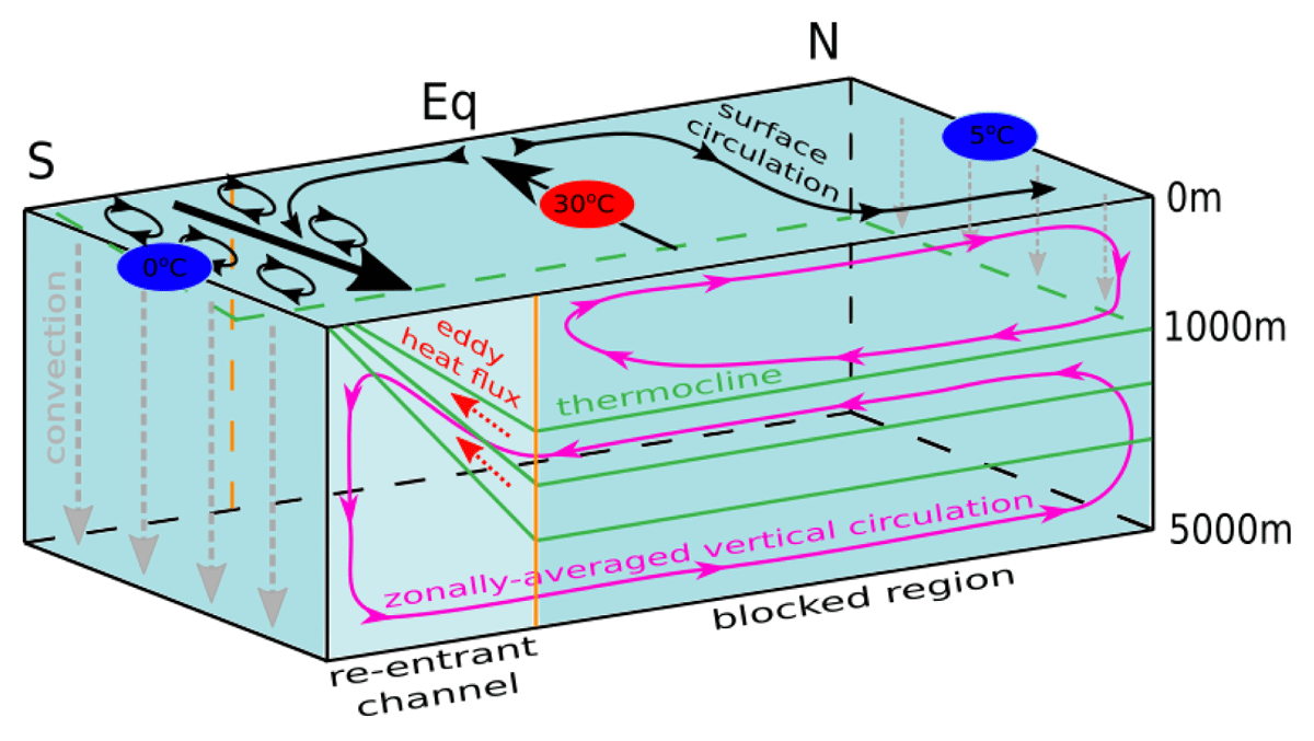
Figure 8
Schematic of thermally-forced circulation. Black arrows indicate the surface circulation, and magenta arrows the zonally-average vertical circulation. Green lines are isotherms, grey dashed arrows indicate convection, and red dashed arrows indicate the eddy heat flux. The orange line marks the northern edge of the re-entrant channel, splitting the re-entrant channel to the south from the blocked region to the north. Numbers in ellipses are the temperatures the ocean surface is restored to, with the red ellipse (at the equator) indicating a region of stabilizing buoyancy flux (heating), and blue ellipses (at the southern and northern boundaries) indicating regions of destabilizing buoyancy flux (cooling).
Our results indicate that Ekman pumping is not required to generate steep density surfaces across the Antarctic Circumpolar Current and to drive a deep-reaching overturning circulation. Previous studies using eddying ocean models have highlighted the role of a zonally re-entrant channel, and the resulting energetic eddy field, in generating mid-depth stratification. This role is via a two-way interaction between southern and northern sinking regions (Wolfe and Cessi 2010, 2011, Shakespeare and Hogg 2012). Our results suggest, however, that the two-way interaction needed to generate a mid-depth stratification does not fundamentally rely on the action of the wind, as assumed in these studies. Of course, this does not mean wind forcing is unimportant, but it means that wind forcing is not necessary to the development of the two-cell overturning circulation as previously assumed. Understanding how, and at which timescales, the wind forcing affects the overturning circulation is left for a separate study.
The crucial role of the channel explains why previous work on the role of horizontal convection on the overturning circulation inferred that buoyancy forcing alone could not generate a deep-reaching overturning circulation without energy input by winds and tides; these studies used either two-dimensional simulations (e.g. Paparella and Young (2002); Ilicak and Vallis (2012)), laboratory experiments (e.g. Wang and Huang (2005); Hughes and Griffiths (2008)) or direct numerical simulations (e.g. Vreugdenhil et al. (2016)) using a basin geometry similar to the blocked domain used here. Consistent with the results presented here for the blocked domain, all these experiments resulted in stratification collapsing to the surface. In the presence of rotation and a re-entrant channel, the overturning circulation is a balance between advection and lateral eddy fluxes along sloping isopycnals, rather than a balance between advection and (mostly) vertical diffusion found for all other cases. This difference might explain why the amount of observed vertical diffusion in the real ocean is insufficient to close the overturning circulation; eddy fluxes compensate for the “missing mixing” in a slantwise direction.
Our results do not contradict those of Sandström (1908), which apply to the thermal layer in a blocked basin, nor the ‘anti-turbulence theorem’ of Paparella and Young (2002), which applies to energy dissipation in the limit of a vanishing vertical diffusivity. In our simulations with weak mixing and a blocked geometry, the thermocline collapses to the surface, as predicted, and consistent with all turbulence-resolving direct numerical simulations in which convection is resolved rather than parameterised. The present results are in line with those of Barkan et al. (2013) and Sohail et al. (2019), who found that buoyancy forcing can drive a deep overturning circulation with a re-entrant domain. In this case the meridional heat transport is carried by eddies which result from baroclinic instability. The latter is an inviscid process and can occur with vanishingly weak mixing. As the eddies are balanced and quasi-two dimensional, the energy cascade can be to larger scales, depending on factors such as bottom drag (Salmon 1980; Vallis 2006).
The present results can be compared with the model of Gnanadesikan (1999), which has a geometry like the present realistic case. In this, the residual transport (from Ekman, minus eddy fluxes) from the Southern Ocean and the transport in the northern region balance upwelling by diapycnal mixing from the interior. While not discussed in the paper, the model admits a solution with a finite thermocline depth in the limit of weak vertical mixing and zero wind stress. Then there is a two way balance between eddy fluxes from the Southern Ocean and transport in the western boundary current in the blocked region. But the model does not specify why the isopycnals are sloping. In our simulations, the sloping isopycnals are due to the presence of convection at the southern boundary, which in turn requires asymmetric temperature forcing at the northern and southern boundaries. Other features in the model of Gnanadesikan (1999) are also probably too simplistic, such as the Munk-like western boundary current (Munk 1950), which neglects the essential role of upwelling and downwelling in the current (e.g. Gjermundsen and LaCasce 2017).
Previous direct numerical simulations examined rotating horizontal convection in blocked or re-entrant domains, but ours employs both, spanning a realistic range of latitudes. Given computational limitations, the deformation radius is barely resolved over the domain. Nevertheless, no eddy parameterisations were employed. Such parameterisations in coarse-resolution models (Gent et al. 1995) can produce unrealistic features, such as an over-sensitivity of the Antarctic Circumpolar Current transport to wind variability (Munday et al. 2013). But even simulations employing eddy parameterizations can exhibit a two-cell overturning with a mid-depth stratification without winds (Munday et al. 2013; Gjermundsen et al. 2018). The key ingredient therefore is the re-entrant channel.
In the present model however, both convection and small-scale mixing are parameterised. Further, the model employs z-levels, which entails numerical diffusion which is impossible to eliminate (Griffies et al. 2000). Appropriate choices for temperature/salinity advection schemes and viscosity can reduce such spurious mixing to acceptable levels (Hill et al. 2012; Ilicak et al. 2012; Megann and Storkey 2021). The present simulations are configured to minimize numerical diffusion under the constraint of keeping numerical runs computationally affordable. We have not attempted to diagnose directly the amount of numerical diffusion as compared to the explicit diffusion used in these simulations. However, if numerical diffusion was dominant in these simulations, there would be little difference in the thermal boundary layer depth between the blocked simulation and those with a channel. We interpret the large sensitivity of the upper cell overturning to increasing prescribed vertical diffusivity (see Figure 6) as proof that numerical diffusion is not dominant, but we cannot discard it having a substantial effect on the lower overturning. But this does not affect the main conclusions of this study.
We also focused on a purely thermally-driven circulation, but salinity of course also plays a major role in the overturning circulation. In northern high latitudes, high salinity is crucial for the formation of warm and salty North Atlantic Deep Water (NADW), that is, the upper overturning cell (Ferreira et al. 2018). The position of the polar transition zone where most of the convection occurs is controlled by a competition between heat and freshwater fluxes (Caneill et al. 2022) which is deeply influenced by nonlinear effects of the equation of state (Roquet et al. 2022). In southern high latitudes, sea-ice ocean interaction plays an important role in the formation of Antarctic Bottom Water (AABW), and hence for the lower overturning cell. In this case brine rejection due to sea-ice production destroys stratification locally, but the freshwater due to the melt of this sea ice increases stratification further north, with the combination of these processes generating the observed vertical structure of the Southern Hemisphere ocean (Klocker et al. 2023). Nevertheless, little is known about the combined effects of heat and freshwater forcing on the global ocean overturning circulation. Experiments on horizontal convection in the presence of freshwater fluxes showing regimes with oscillatory behaviour (Mullarney et al. 2007), bearing some resemblance to those found for glacial-interglacial cycles which occurred in Earth’s past climate. Future work on rotating horizontal convection in a realistic ocean geometry will have to focus on the combined roles of thermal and haline forcings to better understand what sets the observed global ocean overturning circulation.
Appendix A
Scalings for the upper overturning cell
a. Thermal boundary layer thickness
The thermal wind balance holds for the both the horizontal velocities (u, v) as
Based on the scales of the thermal boundary layer thickness δ, the horizontal length scale L, and the velocities U, V, W, we get
The advective-diffusive balance at the bottom of the boundary layer in the thermally equilibrated state suggests
Here, we have neglected horizontal gradients in the boundary layer compared with vertical gradients. We can derive a scaling for the zonal and meridional velocities in terms of boundary layer thickness and diffusivity,
Using (A3) and (A8),
leading to the scaling for the thermal boundary layer thickness, δ,
where Ra is the Rayleigh number, and E is the Ekman number, as defined in Equation 3. This scaling was first given by Welander (1971) (see also Vallis (2006)).
b. Overturning circulation
We now use the scaling for the upper thermal boundary layer to derive a scaling for the strength of the upper-cell overturning circulation.
To derive a scaling for the meridional overturning circulation, Φ, which is equal to the boundary layer transport in meridional direction, ξbl, we first write the meridional velocity as
The transport in the thermal boundary layer per unit width is, therefore
If we assume a basin width of L, this gives a boundary layer transport in meridional direction of
Data Accessibility Statement
The model output can be provided by AK, and requests for the model output should be submitted to ankl@norceresearch.no. The model output shown in Figure 1(a) can be accessed at http://dx.doi.org/10.4225/41/5a2dc8543105a. The data of the observational transect shown in Figure 1(b) can be downloaded at https://cchdo.ucsd.edu/cruise/33RO20161119 (WOCE transect P18).
Acknowledgements
The authors thank Johann Nilsson and Mike Bell for constructive reviews, and AK wants to thank Pål Erik Isachsen and Andy Hogg for useful discussions which helped to improve this manuscript.
Funding Information
Model runs were undertaken with the assistance of resources from the National Computational Infrastructure (NCI), which is supported by the Australian Government. AK and JHL were supported by the Rough Ocean project, number 302743, of the Norwegian Research Council and BG is supported by Australian Research Council Future Fellowship FT180100037.
Competing Interests
The authors have no competing interests to declare.