
Table 1
Available downscaled global coupled models and emission scenarios. The downscaled historical simulations are not the full CMIP5 historical period. Instead they start in the year 1961 and in some cases as late as 1976. All historical simulations, however, end in the year 2005. The RCP scenarios all start in 2006 and end in 2100.
| HISTORICAL | RCP2.6 | RCP4.5 | RCP8.5 | |
|---|---|---|---|---|
| MPI-ESM-LR | X | X | X | X |
| EC-EARTH | X | X | X | X |
| GFDL-ESM2M | X | X | X | X |
| HadGEM2-ES | X | X | X | X |
| IPSL-CM5A-MR | X | X | X | |
| CanESM2 | X | X | X | |
| CNRM-CM5 | X | X | X | |
| NorESM1-M | X | X | X | X |
| MIROC5 | X | X | X | X |
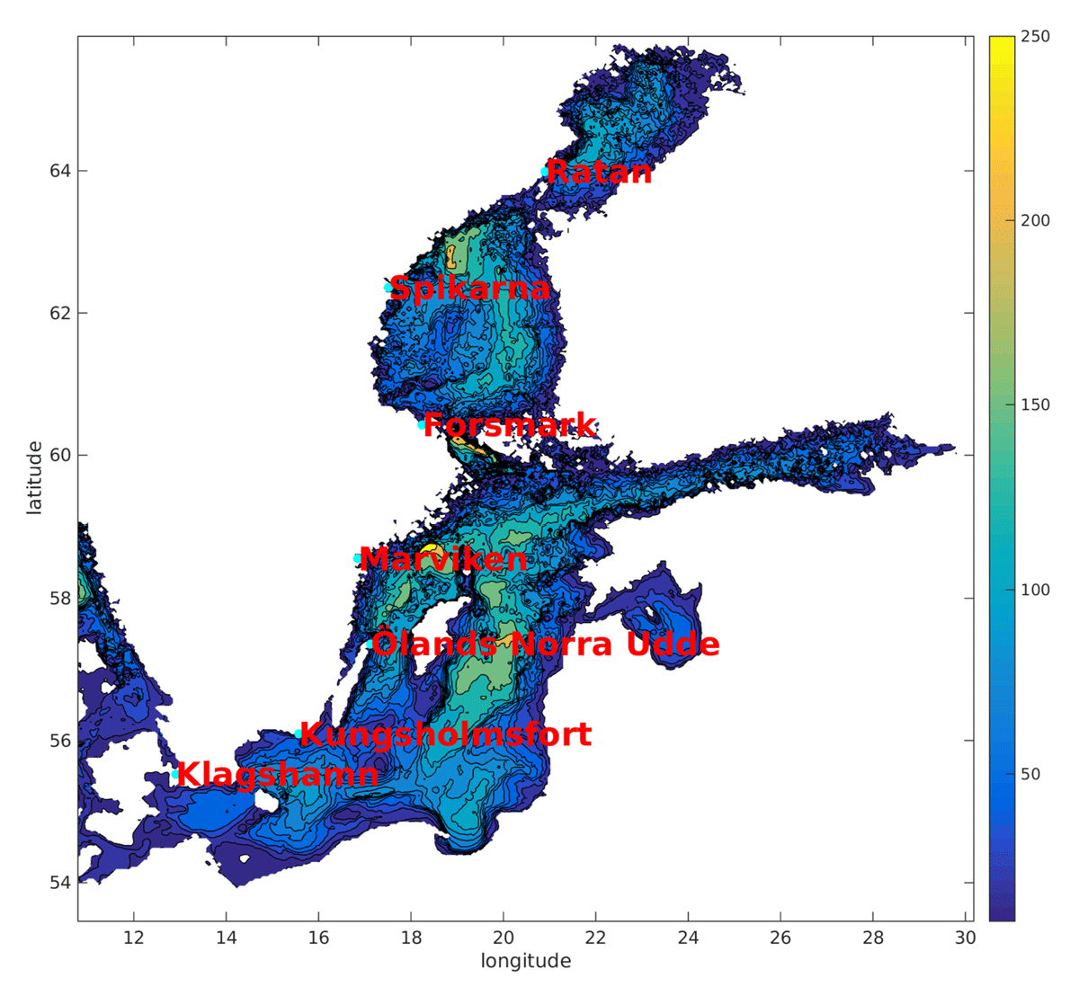
Figure 1
Bathymetric map showing the location of the seven tide-gauge stations used in the study. The colours show the depth in meters.

Figure 2
A schematic of the time delay network. Each hidden layer has five nodes. The time delays differ between the stations and the three iterations. However, for the first iteration we use the last 24 hours at all stations.
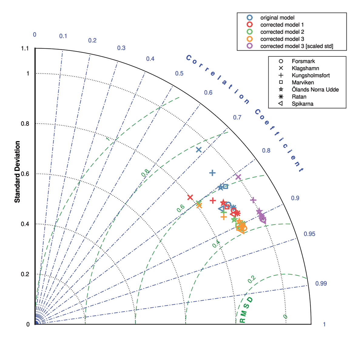
Figure 3
Nondimensional Taylor diagram showing the performance of the RCA4-NEMO (original model) and four versions of the bias corrected model. Both the RMSD and the standard deviations are normalized by the standard deviation of the observed sea level. The best possible performance is thus an RMSD equal to zero, and a correlation coefficient and standard deviation of one.
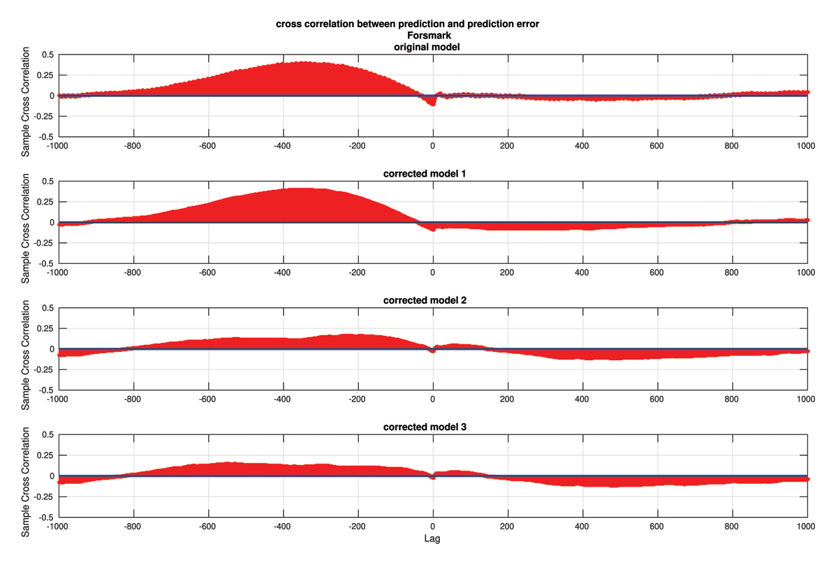
Figure 4
Cross correlation between the model prediction and the prediction error at the station Forsmark. Lags are in hours.
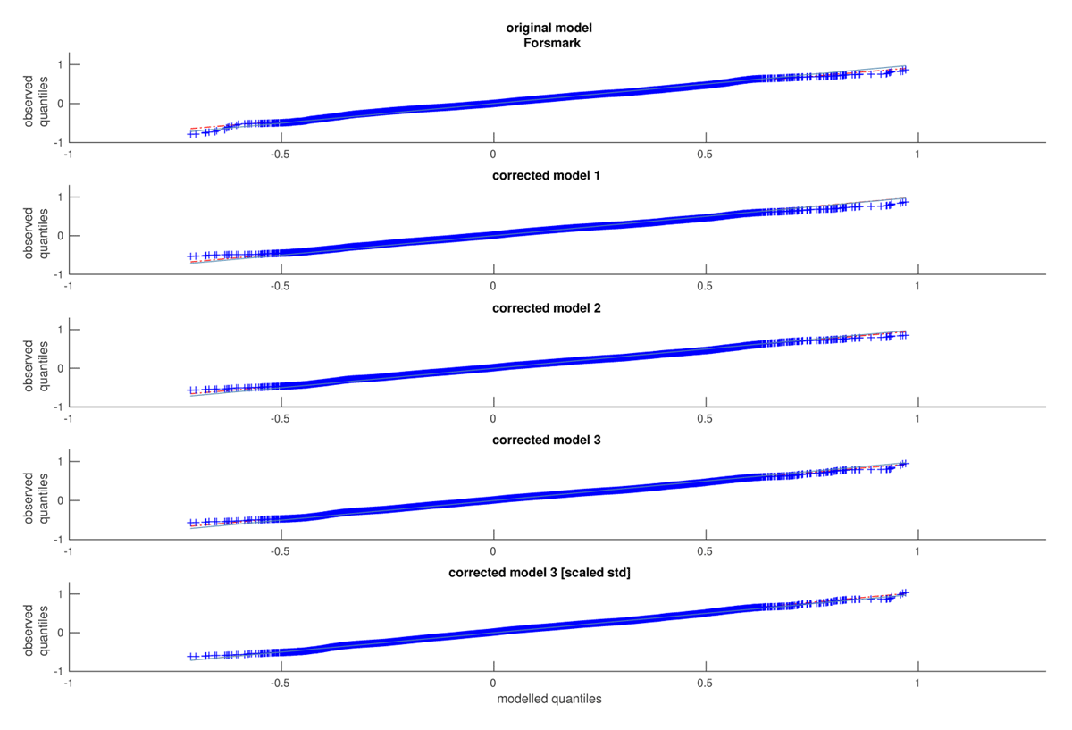
Figure 5
Quantile-Quantile plots for the different models at the station Forsmark. The blue line is one to one, while the dots fall on the red dashed line if the two distributions are the same, but they are scaled and shifted versions of each other.
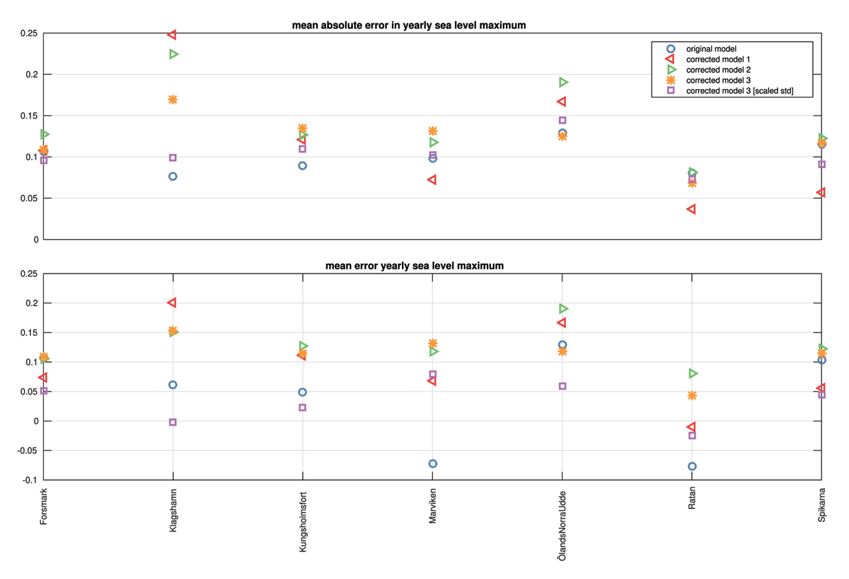
Figure 6
Mean error and mean absolute error of the yearly maxima at the stations. The means are taken over 4 yearly maxima extracted from years starting in July and ending in June.
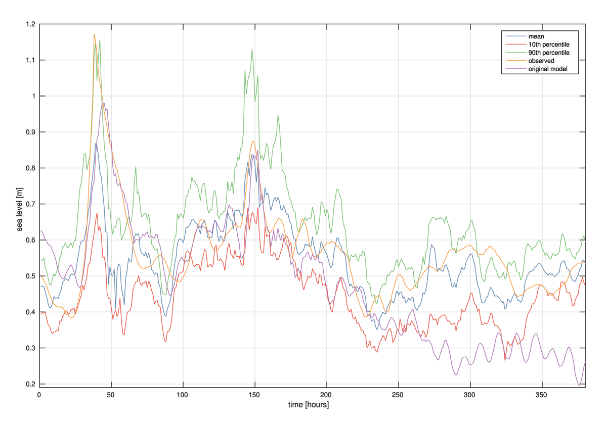
Figure 7
Highest sea level recorded at Spikarna during the period of the test set and its representation in some different models. Mean shows the mean projection from corrected model 3 [scaled std], 10th and 90th are percentiles from the same model ensemble.
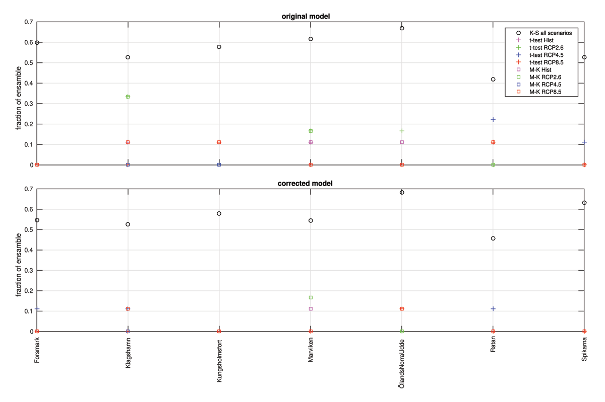
Figure 8
The fraction of the runs per scenario that shows significant trends in yearly sea level maximum. Also shown is the fraction of the ensemble whose yearly sea level maxima could have been drawn from the same distribution. The significance level is 0.05 for all tests. M-K for Mann-Kendall and K-S for the Kolmogorov-Smirnov goodness-of-fit hypothesis test.
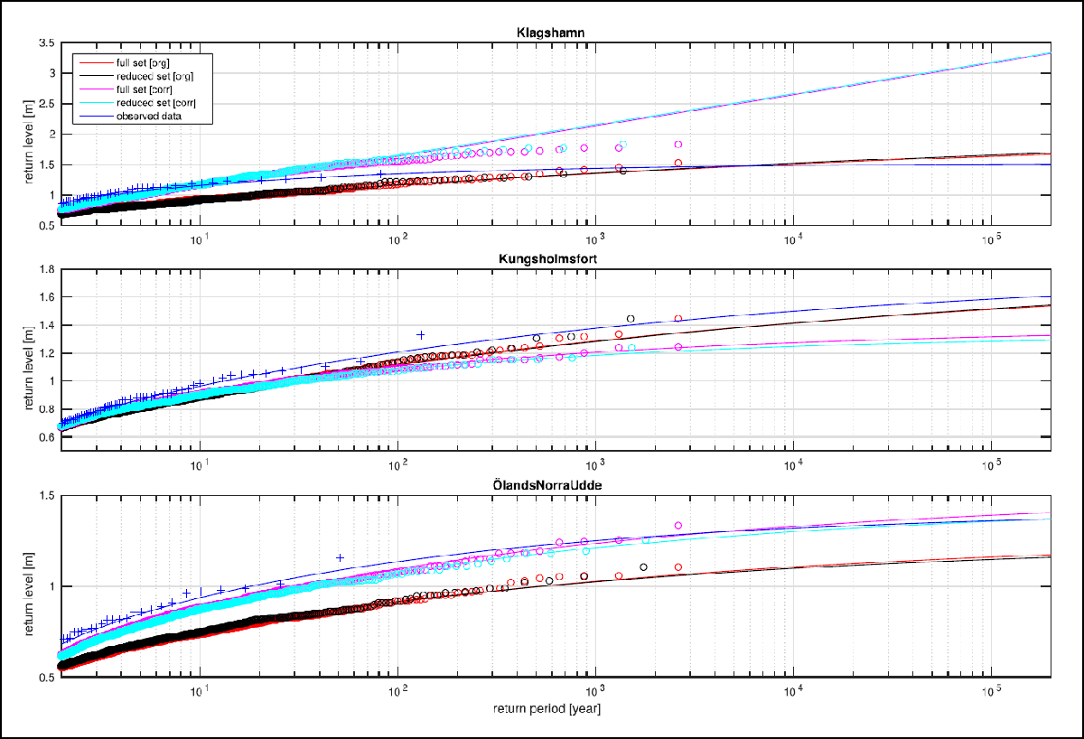
Figure 9
Return level curves for stations Klagshamn, Kungsholmsfort and Öland Norra Udde. All return levels are based on GEV distributions fitted to annual maximum data. The years are defined as running from July to June. The observationally based curve is derived taking the GEV parameters from Hieronymus and Kalén (2020). Rings and pluses show the empirical distributions for modelled and observed data respectively. Full set implies that all 2601 modelled yearly maxima are used. Reduced set is a subset of full where all yearly maxima could have been drawn from the same distribution. The reduced set is derived using the algorithm described in Sect. 4.
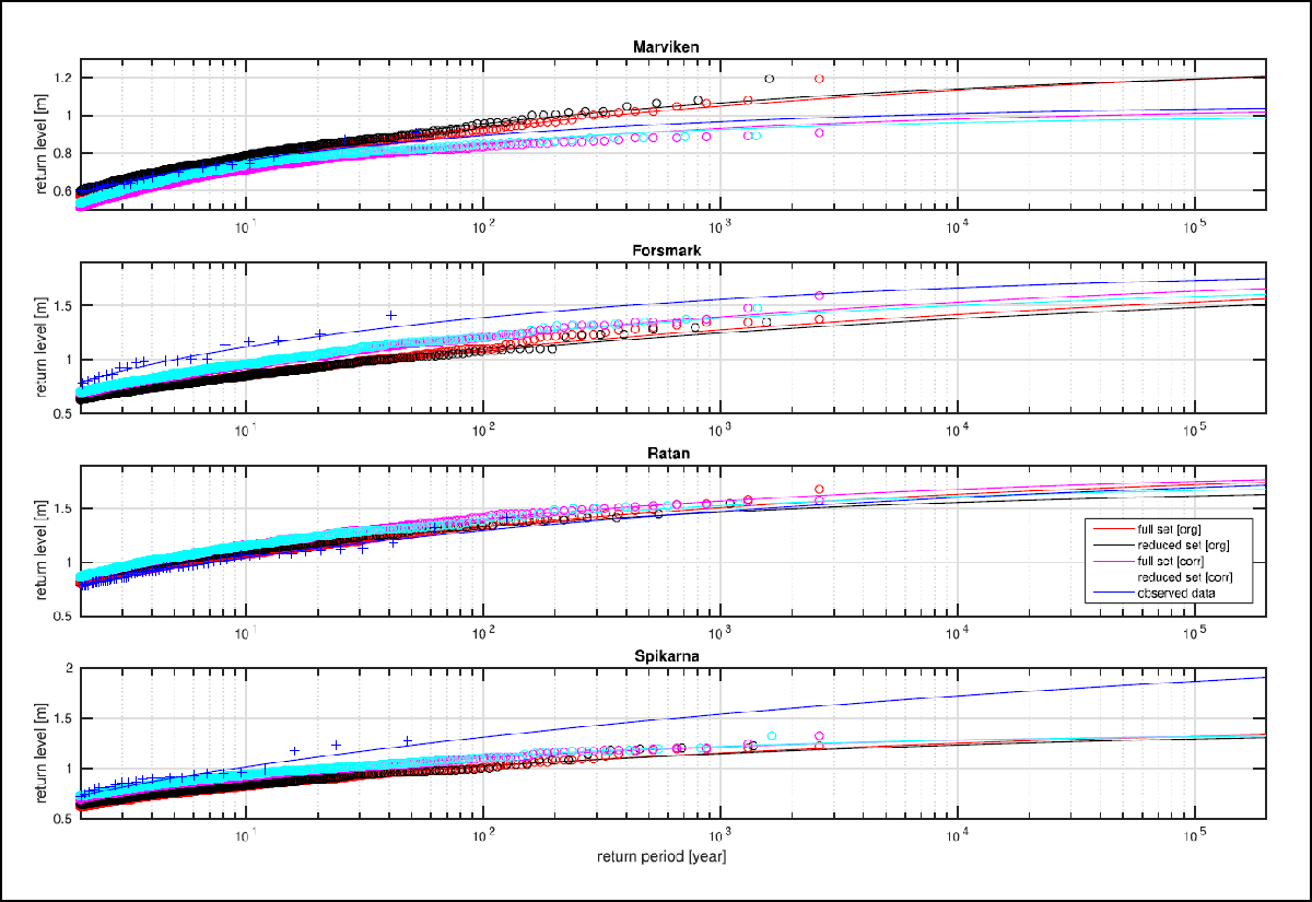
Figure 10
Same as Figure 9, but for stations Marviken, Forsmark, Ratan and Spikarna.
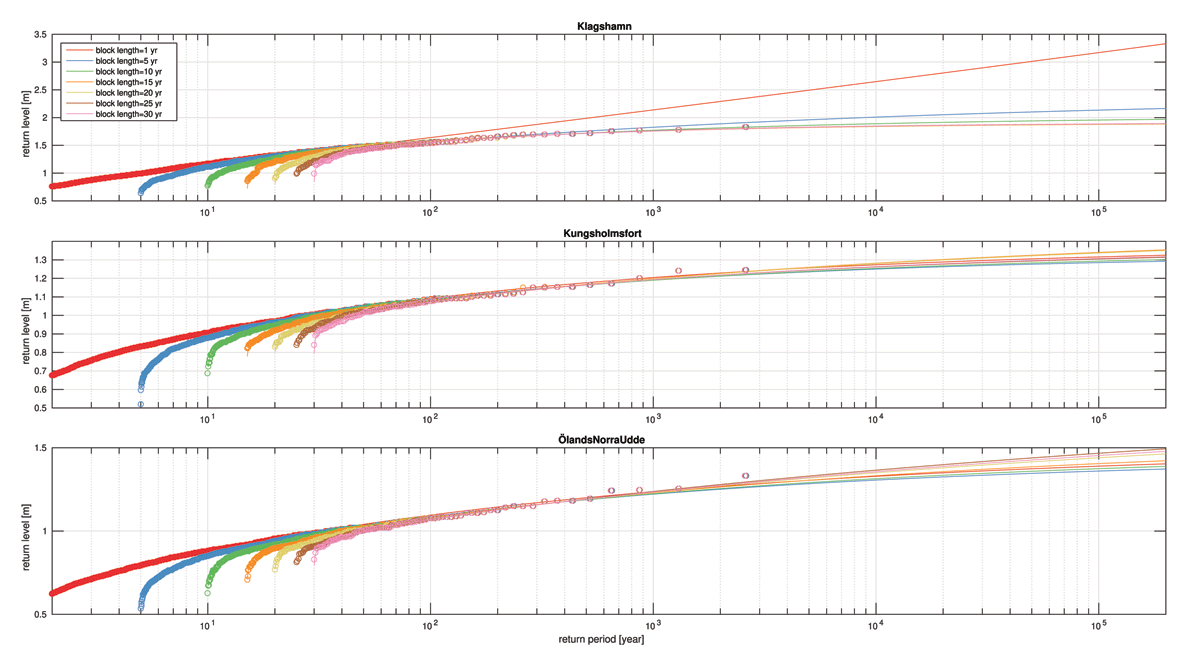
Figure 11
Return level curves for different block lengths for stations Klagshamn, Kungsholmsfort and Öland Norra Udde. The full set of bias corrected data is used in all calculations.
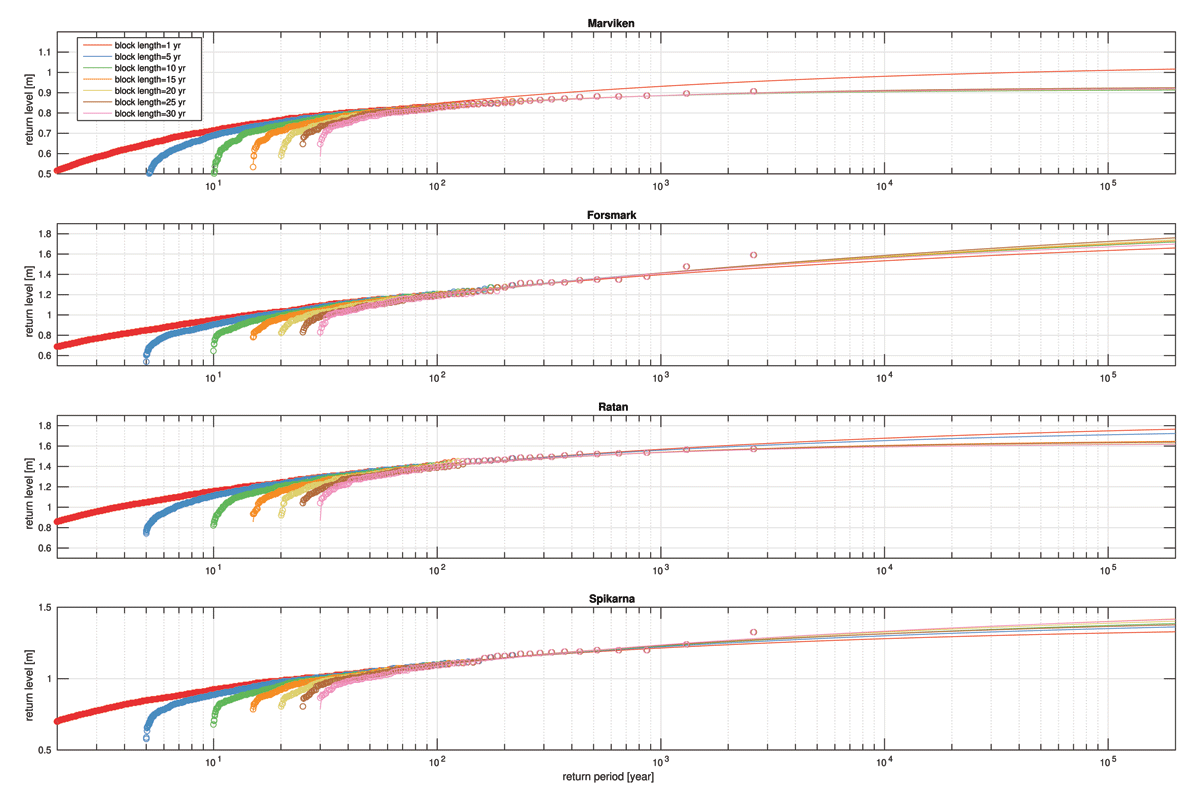
Figure 12
Same as Figure 11, but for stations Marviken, Forsmark, Ratan and Spikarna.