
1 Introduction
Distributions of sea level extremes used in current coastal spatial planning are almost always derived from tide-gauge records. Many of the longest such records in the world come from the Baltic Sea, where a number of time series, with high temporal resolution, exceed 100 years in length (Ekman, 1999; Hieronymus and Kalén, 2020). Nevertheless, these time series are still much too short to give accurate estimates of the often multi-millennial return levels wanted by many coastal spatial planners in support of development plans in coastal areas. Modelled sea level time series that extends for at least thousands of years can on the other hand be produced with relative ease. One may thus ask, why is such data so seldom used for planning purposes? A simple answer to this question is hard to give, but most likely the biggest factor behind the infrequent usage of modelled data in coastal spatial planning is the existence of model biases. Existence of sizeable biases, especially if they affect sea level extremes, can lead to distrust in the modelling systems and render their results unusable for many applications.
Naturally, model biases are not specific to numerical ocean models but exist in all climate models and all variables. Bias correction methods are therefore used as a remedy in a number of scientific disciplines (Teutschbein and Seibert, 2012; Berg et al., 2022). However, bias correction methods, like models, are not perfect (Maraun et al., 2017), but neither are observations. In Sweden today, it is not uncommon that municipalities derive their return levels for sea level from hourly observations taken over perhaps 50 years from some tide gauge that may be located 100 km away from the area the planning is tailored for. It is thus obvious that a model need not be perfect for it to be useful. More precisely, an imperfect modelled record that is much longer and from the correct location is not necessarily inferior to a distant and short observational one.
Our aim here is to introduce a new and powerful bias correction method that we have applied to sea level output from a coupled regional climate model (Dieterich et al., 2019a, b). The current crop of bias correction methods are tailored to correct the distribution of given output variables toward an observationally based distribution of the same variable (Maraun et al., 2017; Berg et al., 2022). These corrections are thus statistical in the sense that they depend only on observed and modelled distributions, not on relationships between the state variables in the model. It is obvious that such statistical corrections have severe limitations. Clearly, biases depend on model states. It follows, that an optimal bias correction strategy cannot be to change the sea level to y m each instant when the modelled sea level is x m.
Our proposed bias correction method is not merely statistical in the sense defined above. Instead it is also physical in the sense that the corrections it calculates are dependent on the state of the model. In practice, we use model states as predictors and observed sea level as a predictand in a nonlinear neural network based regression model. A large part of a model hindcast and concurrent observations are used as training data and a smaller part as a test set. The corrections are then applied to a large number of regional downscalings of global models from the Coupled Model Intercomparison Project – Phase 5 (CMIP5, Taylor et al. (2012)). These global models have been run with a number of different emission scenarios, ranging from strong mitigation under RCP2.6 to very high unmitigated fossil fuel usage under RCP8.5. To our knowledge it is the largest set of downscaled climate scenarios ever produced for the Baltic Sea area.
The dataset is thus an important source of information not only about historical-, but also potential future changes. One important question regarding future sea levels that this dataset could help answer is whether the frequency and/or intensity of storm surges (temporary sea level extremes that occur during severe storms) will be affected by climate change. For planning purposes it is almost always assumed that storm surges are unaffected by climate change, and consequently that future sea level extremes can be estimated by simply adjusting the mean sea level (Hieronymus, 2021; Hieronymus and Kalén, 2022). Trends in sea level extremes have been detected in historical data (Barbosa, 2008; Kudryavtseva et al., 2018). However, it is not clear to what degree these trends are owing to natural variability and anthropogenic climate change respectively. Moreover, it is also not clear to what degree current trends in sea level extremes are owing to changes in storm surges and mean sea levels respectively.
In summary, the manuscript aims to introduce a novel and physically informed bias correction method. The method is applied to hourly sea levels from seven locations around the Swedish Baltic Sea coast, where tide-gauge stations are installed. The primary motivation for developing better bias correction methods for modelled sea levels is to enable a much wider use of modelling data in coastal spatial planning. The primary reason for developing a physical or model state dependent bias correction technique is the obvious fact that model biases are state dependent. Lastly, an auxiliary aim of the manuscript is to investigate storm surge variability, forced as well as natural, using what is presumably the largest set of downscaled ocean-atmosphere data ever produced for the Baltic Sea area.
2 Models & Data
2.1 Coupled climate model
The model data used in this study derives from dynamical downscalings of global coupled climate models from CMIP5 (Taylor et al., 2012), with the regional coupled atmosphere-ocean-sea ice model RCA4-NEMO (Jeworrek et al., 2017; Dieterich et al., 2019a, b; Gröger et al., 2019). RCA4-NEMO consists of the atmospheric model RCA4 (Samuelsson et al., 2011; Berg et al., 2013) and the ocean-sea ice model NEMO-Nordic (Madec and the NEMO team, 2016; Hordoir et al., 2018). The atmospheric grid covers Europe and parts of the North Atlantic, with a horizontal resolution of 25km and with 40 vertical levels. The ocean grid covers the North Sea and the Baltic Sea with a horizontal resolution of 3.7 km and with 56 vertical levels. The model system as a whole is thus partially coupled. However, over our area of interest, the Baltic Sea, it is fully coupled. Outside of the coupled regions the atmospheric model is forced with SSTs from the driving global climate models.
A large ensemble of global coupled models forced with greenhouse gases and aerosols from different representative concentration pathways (RCPs) (van Vuuren et al., 2011) have been downscaled, over many years, using RCA4-NEMO at the Swedish Meteorological and Hydrological Institute (SMHI). A full list of the different runs is given in Table 1. In addition to the downscaled climate projections, a downscaled ERA-Interim (Dee et al., 2011) forced hindcast is also available with the same RCA4-NEMO model system. The hindcast covers the years 1979-2012 and it is here used as training data for the neural network regressions.
Table 1
Available downscaled global coupled models and emission scenarios. The downscaled historical simulations are not the full CMIP5 historical period. Instead they start in the year 1961 and in some cases as late as 1976. All historical simulations, however, end in the year 2005. The RCP scenarios all start in 2006 and end in 2100.
| HISTORICAL | RCP2.6 | RCP4.5 | RCP8.5 | |
|---|---|---|---|---|
| MPI-ESM-LR | X | X | X | X |
| EC-EARTH | X | X | X | X |
| GFDL-ESM2M | X | X | X | X |
| HadGEM2-ES | X | X | X | X |
| IPSL-CM5A-MR | X | X | X | |
| CanESM2 | X | X | X | |
| CNRM-CM5 | X | X | X | |
| NorESM1-M | X | X | X | X |
| MIROC5 | X | X | X | X |
The coupled model has been described in great detail and validated extensively (see e.g. Jeworrek et al. (2017); Dieterich et al. (2019a, b); Gröger et al. (2019)). Our focus here is on sea level variability. The performance of the coupled model on classical skill scores such as correlation coefficient and root mean square error is considerably worse than for similar uncoupled ocean configurations. The purpose of the bias correction method here introduced is thus to improve the model’s ability to represent sea level variability. Our validation of model performance is presented together with our validation of the performance of the bias correction method in Sect. 3.
The observed sea level data come from the Swedish tide-gauge network (SMHI, 2022). Data from seven stations are used, and those stations were chosen because they have full data coverage for the years the ERA-Interim driven hindcast is available. The location and names of these seven stations are shown on the map in Figure 1. All sea level data, modelled as well as observed, is hourly and all time series are linearly detrended to remove the effects of land uplift and mean sea level change. Our focus here is thus on high rather than low frequency sea level variability. This focus is partly owing to our interest in extreme events such as storm surges. However, it is also a direct consequence of the limitations of the modelling system which lacks ice-sheet-, global ocean- and glacial isostatic adjustment components. In other words, the main drivers of mean sea level change in the area are not described by the modelling system. The tidal range is small but non-zero at our seven stations. Following Hieronymus et al. (2019), we opted to keep the tidal signal in both the observational and modelled data. The bias correction method is thus set-up to correct errors of tidal as well as other origins.
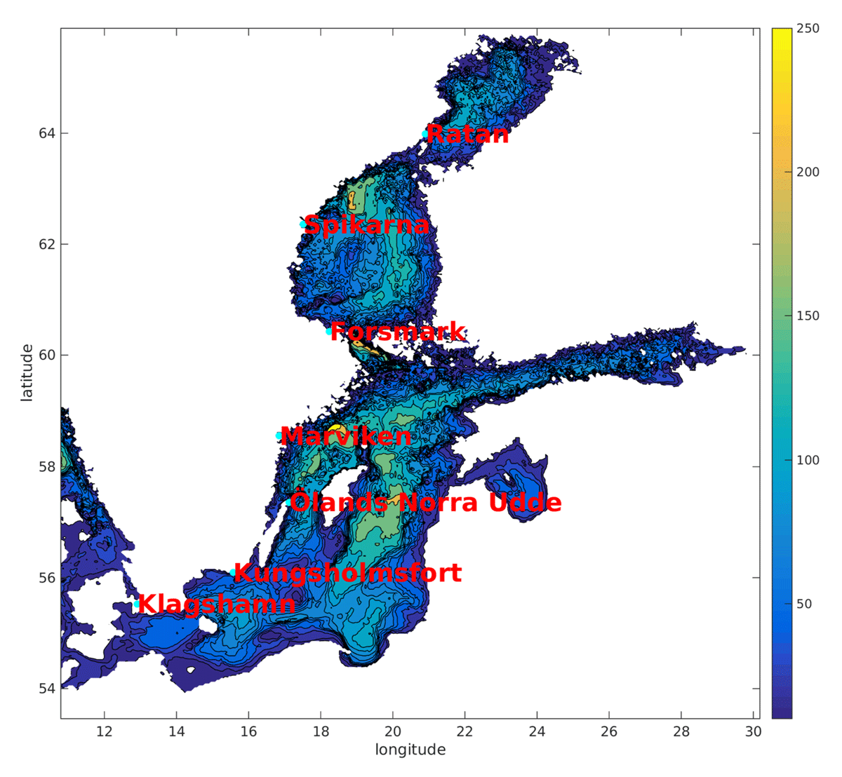
Figure 1
Bathymetric map showing the location of the seven tide-gauge stations used in the study. The colours show the depth in meters.
2.2 Machine learning model
The time delay neural network from Matlab’s deep learning toolbox is used for the bias correction. This particular network was tested on several different sea level regression problems by Hieronymus et al. (2019). The architecture of the network used in this earlier study was, however, less elaborate than the one used here. Figure 2 shows a schematic of the current architecture. The network features an input layer, three hidden layers and one output layer. The network used by Hieronymus et al. (2019), for comparison, had only one hidden layer. The input variables, x(t), are fed from the input layer into a time delay that in turn feeds a number of time steps through to the first hidden layer. The number of past time steps of x(t) used to predict y(t) is determined by the user. Here we start by feeding data from the last 24 hours into the system. An iterative procedure is then used to improve on the delays as described in Sect. 3.

Figure 2
A schematic of the time delay network. Each hidden layer has five nodes. The time delays differ between the stations and the three iterations. However, for the first iteration we use the last 24 hours at all stations.
Every hidden layer contains five hidden nodes. Each hidden node calculates a linear combination of its input variables, using weights that are determined through a training procedure. This linear combination is then used as an argument for a sigmoid function, and the transformed signal is sent to the next layer. The last layer the signal reaches is the output layer, which has a linear activation function instead of sigmoid one, so that an unbounded range of values can be predicted.
As stated previously; training the network amounts to finding suitable weights to use for the linear combinations calculated by the different nodes. These weight are initialized randomly, and the Levenberg-Marquardt backpropagation algorithm is used iteratively to find weights that minimizes the mean square error between the prediction and the target. The training and target data is subdivided into a training and a test set. The test set is approximately the last five years of the data, and all plots showing network performance in this article are based on the test set. The training set is also subdivided into a training, test and validation part. Early stopping is implemented into the iterative Levenberg-Marquardt backpropagation algorithm to avoid overfitting. In practice this means that when the performance on the validation part of the training set starts to deteriorate, the network training is discontinued.
Both the input data (x(t)) and the output data (y(t)) of the neural networks are transformed as part of the pre-processing and post-processing. The input data are transformed using singular value decomposition and only the time dependent parts, the so called principal components, are used as inputs. The model variables used as input data are meridional and zonal winds and sea level. Each model variable is taken from a small sub-set of grid points in the model, to minimize the otherwise enormous amount of input data. All input data is hourly and the modelled sea levels are detrended just as the observed sea levels. The input data are arranged into an m × n matrix M, where m is the number of input variables and n the number of time steps. A singular value decomposition is then applied to M, giving
where the columns of U are the empirical orthogonal functions, L is a diagonal matrix that holds the squared eigenvalues of the spatial covariance matrix and VT holds the principal components (Calafat and Jordá, 2011). Putting A = UL, where A is determined from the training data and kept the same for all subsequent applications, we can recreate the variables in M at the time step t through.
where m = M(t) is the column vector of M that corresponds to the time t and x̃ = VT(t) is a vector of principal components corresponding to the same time step. The principal components used to forced the neural network can thus be found for any timestep from any run through
The first 17 principal components in x̃ are then used as input to the neural networks. Our 18th and last input variable is the modelled sea level from the station the neural network is set-up to correct. These inputs are then further transformed through
where x̃ here incorporates also the 18th input variable and the overline operator signifies that it is the time mean of the variable taken over the training period. That is,
where N is the total number of time steps in the training period. The observed sea levels (SSH(t) i.e. our targets for the network training) are similarly transformed according to
The outputs of the neural network, the corrected sea levels, are thus found from
Each neural networks predicts sea level from a single station, and we use an ensemble of 30 networks for each station. A total of 210 network are hence trained to correct sea level at our seven stations. The ensemble mean over all 30 members of SSHcorr(t) is used as our corrected model prediction.
3 Performance of the bias correction method
A number of different numerical ocean models have been, and are currently, used at SMHI to predict sea levels. In the Baltic Sea, the performance of such models is often extremely good. For the uncoupled NEMO-Nordic model (Hordoir et al., 2018) in hindcasts, correlation coefficients between modelled and observed sea levels are typically around 0.95. In a very simplified and uncoupled barotrophic version of NEMO-Nordic the hindcast correlation coefficients are typically larger than 0.9 (Hieronymus et al., 2017, 2018). Moreover, using machine learning techniques Hieronymus et al. (2019) demonstrated correlation coefficients in excess of 0.99 for some Baltic Sea stations. The correlation coefficient for RCA4-NEMO at our seven stations on the test set data range from 0.68 to 0.86, see Figure 3. The RCA4-NEMO model thus performs considerably worse on these metrics than other similar models, which is also one of the reasons it was chosen as our test case for this new bias correction method.
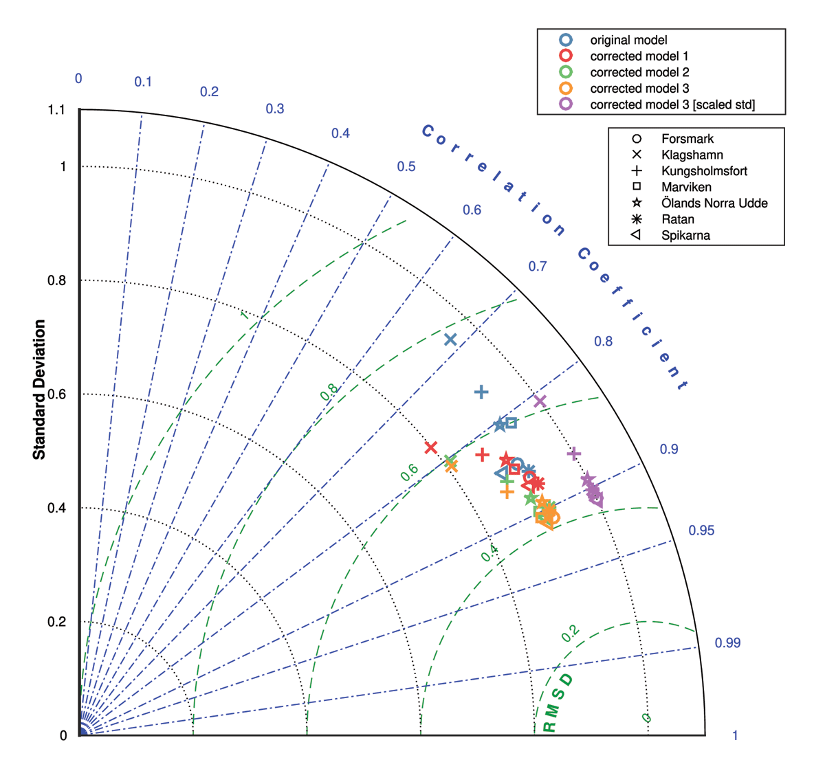
Figure 3
Nondimensional Taylor diagram showing the performance of the RCA4-NEMO (original model) and four versions of the bias corrected model. Both the RMSD and the standard deviations are normalized by the standard deviation of the observed sea level. The best possible performance is thus an RMSD equal to zero, and a correlation coefficient and standard deviation of one.
As noted earlier, the neural networks have a user specified time delay. Tuning the time delay is an efficient way to increase model performance. Here we use an iterative process to find a suitable time delay. The first iteration of the bias correction model (corrected model 1) uses the last 24 time steps (the last 24 hours) of the input variables as predictors. Figure 4 shows the cross correlation between the prediction and the prediction error of the different models at the station Forsmark. For iteration 2 (corrected model 2) we added five time steps around the lag with maximum correlation (i.e. around -390 in the case of Forsmark) as inputs, and removed five time steps from the earlier time delay. A whole new ensemble (corrected model 2) was then trained with the new delays. The second iteration gave a considerable improvements in the performance (see Figure 3) and a similarly substantial reduction in the cross correlations shown in Figure 4. A third iteration (corrected model 3) was then done where three time steps around the maximum correlation (i.e. around -200 in the case of Forsmark) was added and three of the delays from the first iteration was removed. The performance was again improved and the cross correlation was lessened. However, the changes from iteration two to three are much smaller than from iteration one to two. Corrected model 3 has a correlation coefficient exceeding 0.9 at four out of seven stations, while the lowest correlation coefficient in the set is 0.81. Given the good performance and the diminishing returns, a fourth iteration was not performed.
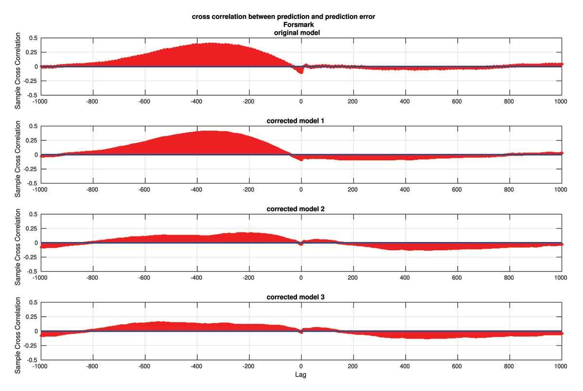
Figure 4
Cross correlation between the model prediction and the prediction error at the station Forsmark. Lags are in hours.
The standard deviations (std) of the sea level from both the different corrected models and the original model are all too low compared to the observed std. Getting the std to agree with observations can be achieved through a simple rescaling of the model outputs. We therefore introduce our final bias correction model, corrected model 3 [scaled std], which has its output scaled to have the same std as the observations. The scaling does not affect the correlation coefficient, but it does increase the RSMD a little as can be seen in Figure 3.
The performance on higher percentiles is typically improved by the scaling. Figure 5 shows quantile-quantile plots for the different models at the Forsmark station. It is clear from the figure that all iterations of the bias correction model give too high sea levels for the lowest quantiles. It is also clear that the original model underestimates the highest quantiles and that those are much improved especially in corrected model 3 [scaled std]. The ability of the different models to represent the yearly sea level maxima over the test set is shown in Figure 6. Both the mean error and mean absolute error is shown. Corrected model 3 [scaled std] is clearly the best in terms of mean error, which is very close to zero at all stations. The original model has the lowest absolute error when an average is taken over all seven stations, but the mean absolute error in the corrected model 3 [scaled std] is only 0.0029 m larger, so the difference is clearly not significant. Overall it is clear that the performance on the test set is better for corrected model 3 [scaled std] than for the other models. This model is therefore our bias correction model of choice and the only one used henceforth.
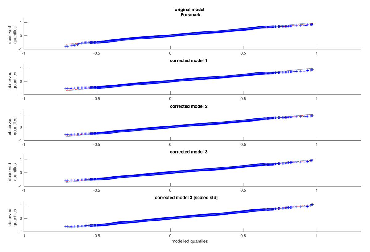
Figure 5
Quantile-Quantile plots for the different models at the station Forsmark. The blue line is one to one, while the dots fall on the red dashed line if the two distributions are the same, but they are scaled and shifted versions of each other.
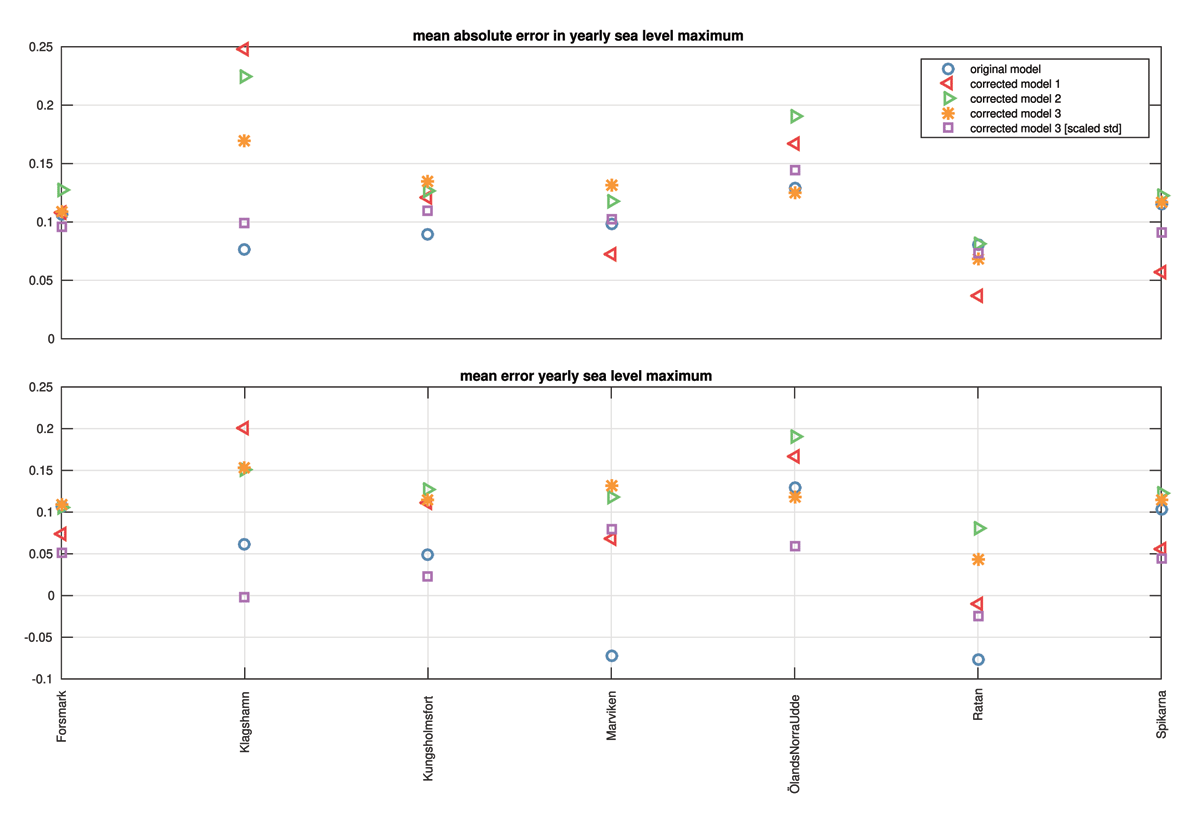
Figure 6
Mean error and mean absolute error of the yearly maxima at the stations. The means are taken over 4 yearly maxima extracted from years starting in July and ending in June.
The ensemble approach of having 30 networks predicting sea levels at each station does not only improve the prediction, it also allows for uncertainty quantifications. Figure 7 shows the 10th, 90th and mean projection from corrected model 3 [scaled std] as well as the original model and the observed sea level during the period of the test set when the highest sea level was measured at the station Spikarna. Here we find the observed sea level to typically be within the 10th to 90th percentile range of the bias corrected data. However we also find this range to be much wider during times when the sea level is very high than during times when sea levels are lower, indicating the obvious fact that sea level maxima are more uncertain than lower percentile sea levels. Moreover, the width of a percentile range produced by the bias correction model ensemble can be used as a quantitative measure of the accuracy of the model prediction. Such a measure is hard to get without using an ensemble prediction system.
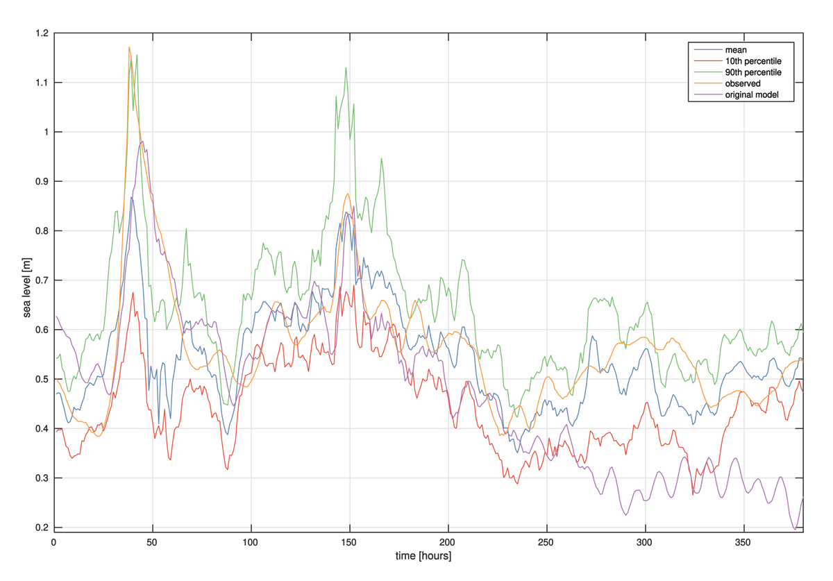
Figure 7
Highest sea level recorded at Spikarna during the period of the test set and its representation in some different models. Mean shows the mean projection from corrected model 3 [scaled std], 10th and 90th are percentiles from the same model ensemble.
4 Trends in storm surges
The presence of trends in the yearly sea level maxima in the different runs is investigated using two methods that are applied both to the corrected and original data. Note that both modelled and observed hourly sea level data are detrended to remove long term trends in sea level and vertical land motion. Any remaining trend in yearly sea level maxima we therefore ascribe primarily to changes in storm surge intensity or frequency, which is our focus here. We note, however, that mean sea level change is not linear in time and thus that residual trends may also owe partly to mean sea level change.
The first trend detection method is a t-test of the slope coefficient of a linear trend estimate and the second is a Mann-Kendall test. The same significance level of 0.05 is used in both cases. Figure 8 summarizes the results. There is a good agreement between the two tests, and only a small fraction of runs show significant trends under any emission scenario. The agreement is also good between corrected and uncorrected data in terms of the fraction of significant trends, although the fraction is smaller for the corrected data. It is important to note that the small fraction of significant trends in itself does not prove that yearly sea level maxima are independent of, or only very weakly dependent on, climate change. However, the lack of a dose-effect relationship, suggests that climate change is not a main driver of the detected trends. That is, significant trends are not more common under the very high emission scenario RCP8.5 than under the other scenarios. Suggesting that natural variability rather than forced changes is a more likely candidate for explaining those significant trends that were indeed found.
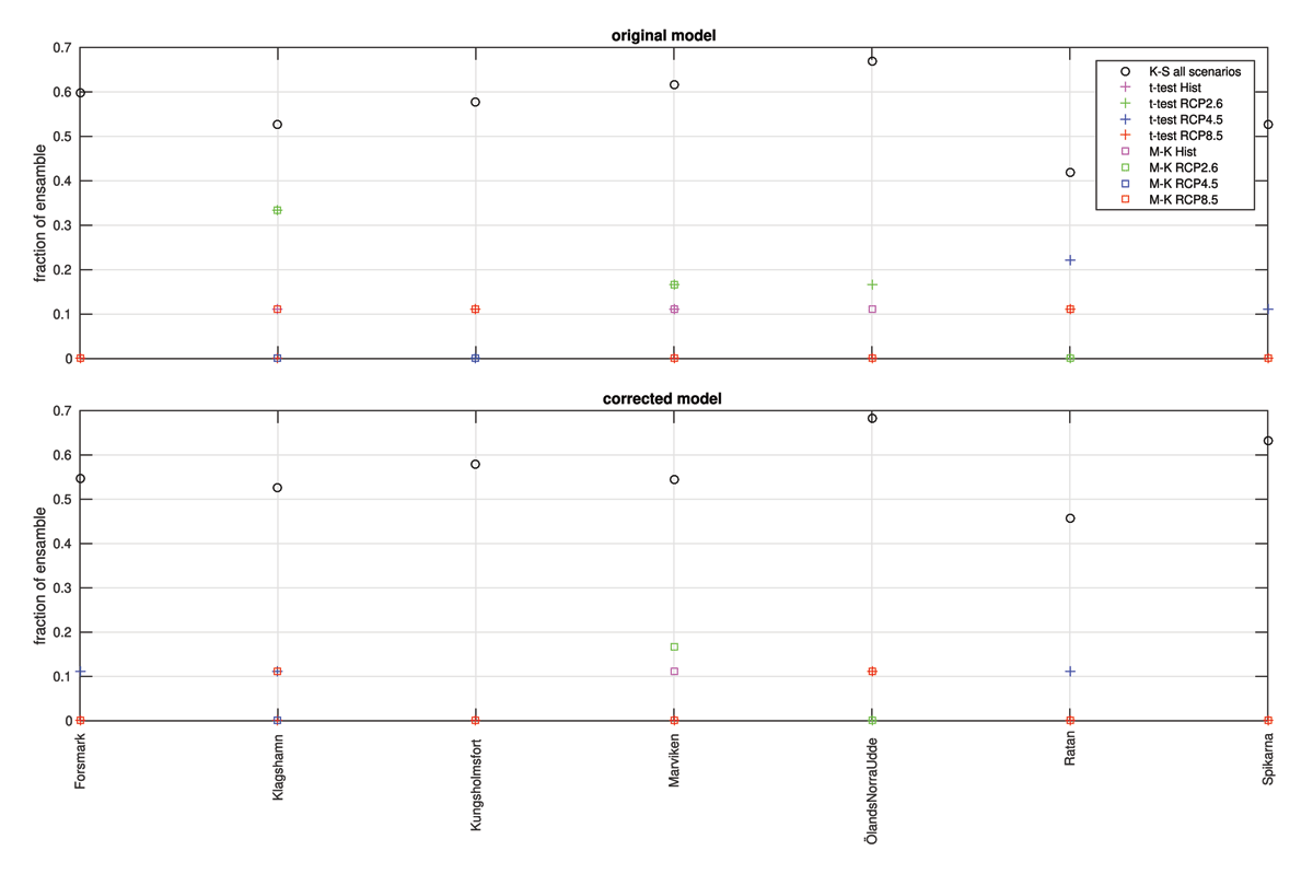
Figure 8
The fraction of the runs per scenario that shows significant trends in yearly sea level maximum. Also shown is the fraction of the ensemble whose yearly sea level maxima could have been drawn from the same distribution. The significance level is 0.05 for all tests. M-K for Mann-Kendall and K-S for the Kolmogorov-Smirnov goodness-of-fit hypothesis test.
Bias correction methods have sometimes been found to deteriorate trends (Cannon et al., 2015), and some trend preserving bias correction methods have been introduced as a remedy (Lange, 2019; Berg et al., 2022). For our particular method, which is based on relationships between physical parameters rather than on relationships between modelled and observed distributions, we have no a priori reason for expecting trends in high quantiles like yearly maxima to deteriorate. However, with the data we have today we can only conclude that the number of significant trends is not very different between the original and corrected model.
Another way to test how different the yearly maxima in the different simulations are is to test whether samples from different simulations could have been drawn from the same distribution. To do so two-sample Kolmogorov-Smirnov goodness-of-fit hypothesis tests are performed on all yearly maximum sample pairs. A large subset of yearly maxima is then constructed by putting together yearly maxima from runs where the null hypothesis that the samples could have been drawn from the same distribution is not rejected. In practise we use a simple and fast heuristic method of our own invention to find this subset from all samples. The subsets produced always contain a large part of the full set of samples, but it may not always converge to the biggest possible subset. The method is as follows. First the samples are arranged in a vector , where each Ym is a set of yearly maxima from one simulation. The short historical simulations have the lowest indices followed by the RCP2.6, RCP4.5 and RCP8.5 simulations. A symmetric matrix is then constructed according to
where if the null hypothesis that the samples could have been drawn from the same distribution is rejected, otherwise . A iterative elimination procedure is then initiated by successively eliminating the row and column with the most ones. In case multiple row-column pairs have the same amount of ones in them we eliminate the one with the lowest index first, so that the short historical simulations are preferentially eliminated. After a number of iterations the matrix contains only zeros and the runs corresponding to the remaining columns of the matrix constitute a large set of yearly maxima that could have been drawn from the same distribution at the chosen significance level of 0.05.
The results of the heuristic method are shown in Figure 8, and are very similar for corrected and uncorrected values. For our seven stations the algorithm typically finds that a little more than 50% of the data could have come from the same distribution. In terms of samples the algorithm finds that between 15 and 22 out of 33 total samples, depending of the station, could have come from the same distribution for the original model data. For the corrected model data the numbers are between 16 and 23 out of 33 samples, and the stations with the most and fewest samples are the same for both data sets. Furthermore, all subsets found using the heuristic method contain samples from all emission scenarios. That is, at all stations we find samples from the historical simulations that the method cannot exclude having been drawn from the same distribution as samples coming from RCP8.5 simulations. Given the very high emissions and strong warming projected under RCP8.5 compared to the historical period, this result again suggests that trends in storm surges are more likely due to natural variability than to anthropogenic climate change.
5 Return levels
The absence of a dose-effect relationship for trends in yearly maximum sea level with emission levels, the small number of trends detected overall and the fact that we could not exclude that a large subset of the whole ensemble of yearly maximum samples could have been drawn from the same distribution, together suggests that the yearly maximum samples from the different scenarios could be grouped together. By so doing, very long datasets can be formed. This method has been tested before by Särkkä et al. (2017) who grouped together sea level data from many different climate scenarios to form one 850 year long time series. Such datasets can tell us something about the frequency and amplitude of very rare storm surge events, i.e., events that are too rare to occur in most observational records.
Two different long datasets are produced: the first called “full set” contains all the yearly maxima from all downscaled models and scenarios, the second called “reduced set” contains the subsets produced by the heuristic method. A generalized extreme value (GEV) distribution (Coles, 2001) is fitted to both these sets for the corrected as well as the uncorrected values. Return levels for the different stations based on these GEV fits as well as observationally based return levels from (Hieronymus and Kalén, 2020) are shown in Figures 9 and 10. A first noteworthy observation is that the difference between the full and the reduced set is negligible at all stations. Given that the climate, and indeed also the general circulation, is very different in the different historical and RCP scenarios it gives further support to the notion that storm surges are not strongly affected by climate change, at least, not in the modelling world.
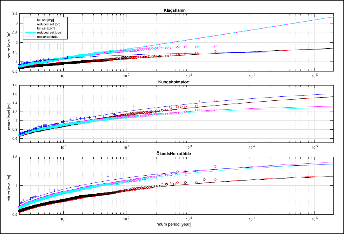
Figure 9
Return level curves for stations Klagshamn, Kungsholmsfort and Öland Norra Udde. All return levels are based on GEV distributions fitted to annual maximum data. The years are defined as running from July to June. The observationally based curve is derived taking the GEV parameters from Hieronymus and Kalén (2020). Rings and pluses show the empirical distributions for modelled and observed data respectively. Full set implies that all 2601 modelled yearly maxima are used. Reduced set is a subset of full where all yearly maxima could have been drawn from the same distribution. The reduced set is derived using the algorithm described in Sect. 4.
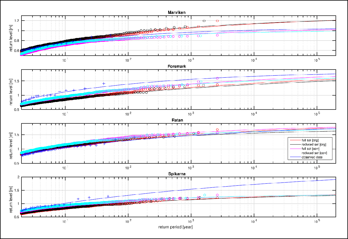
Figure 10
Same as Figure 9, but for stations Marviken, Forsmark, Ratan and Spikarna.
It is also clear to see that even with the corrections in place there are still stations that deviate considerably from the observations. There are also at least one stations, Kungsholmsfort, that appears to have better return levels in the uncorrected model. The same is likely true also about Marviken at least for very high return periods. The highest observed sea level in the 51 year long time series at Marviken is 0.91 m, which is the same as the maximum value of the 2601 year long corrected time series. So it seems very likely that the corrected model underestimates the extremes at Marviken. On the other hand, the difference in a 100000 year return level at Marviken between corrected and uncorrected values is only about 0.2 m. Coincidentally, Marviken and Kungsholmsfort are also the only two stations where the original model’s return levels are higher than those based on the corrected values. Indicating that the predominant problem with the model’s yearly maximas is a low bias, and consequently that a successful bias correction should produce higher yearly maxima.
Another noteworthy feature is that the return level curves typically fit extremely well for short return periods, and less well for long periods. This can be improved upon by fitting GEV distributions to longer than annual blocks. The usage of the GEV distribution is motivated by the Fisher-Tippett-Gnedenko theorem, which states that block maximum of samples can only converge in distribution to the GEV distribution. Block lengths of one year are typically used, but this is only because one year is the smallest block length where one can reasonably assume the extracted maxima to be independent and equally distributed. With thousands of years of data we can afford to use longer blocks. Return level curves for different block lengths are shown in Figures 11 and 12. The longer block lengths notably improve the fits at Klagshamn and Marviken. Especially for Klagshamn where the difference in a 100000 year return level exceeds 1 m and the fit to modelled annual maxima is very poor for return periods longer than 100 years. For Klagshamn it is the shape parameter of the GEV distribution that is affected. With yearly blocks we get a positive value. A positive shape parameter means that the data is Fréchet distributed and has a very heavy right tail. All other fits including that from Klagshamn with longer blocks gives negative shape parameters and are thus Weibull distributed. The Weibull distribution has a much weaker right tail than the Fréchet distribution. Weibull distributed storm surges is also consistent with earlier work from both Sweden and Finland (Räty et al., 2022; Hieronymus and Kalén, 2022).
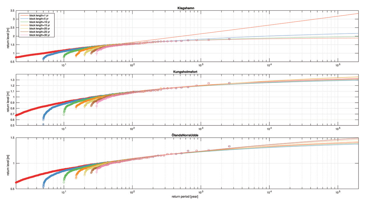
Figure 11
Return level curves for different block lengths for stations Klagshamn, Kungsholmsfort and Öland Norra Udde. The full set of bias corrected data is used in all calculations.
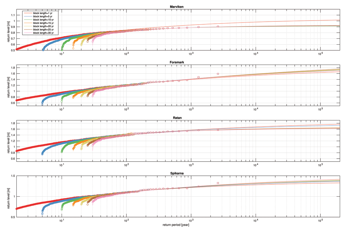
Figure 12
Same as Figure 11, but for stations Marviken, Forsmark, Ratan and Spikarna.
An interesting sidenote is that earlier studies (Dangendorf et al., 2016; Hieronymus and Kalén, 2020) found observationally based return level curves to be sensitive to single high yearly maxima being added or subtracted from the record. Here we find a instead a large sensitivity to having many low or medium values for the Klagshamn station. This is somewhat at odds with the commonly held view that many observationally based return level curves may be biased low owing to a lack of very extreme yearly maxima in short observational records (Dangendorf et al., 2016; Fredriksson et al., 2016; Hieronymus and Kalén, 2020; Hieronymus and Hieronymus, 2021). In conclusion, this sensitivity again strengthens the case for using long modelled time series to constrain return levels from short observational records.
6 Conclusions
A new machine learning based bias correction method is presented. The method is physical in the sense that its bias corrections are dependent on the states of the model it corrects. Current bias correction methods are almost always purely statistical, in the sense that they operate only on the distributions of modelled variables. A physical method has many advantages; notably it would be very unlikely to get great improvements in classical skill scores such as correlation coefficients and root mean square errors from a purely statistical method. There are, however, also some weaknesses. For the method to work one must have a model that can be run in hindcast mode. For example a regional model or global ocean only model. However, a global coupled atmosphere ocean model cannot readily be run in hindcast mode. Thus, the range of models the physical bias correction method can be applied to is smaller than for purely statistical methods.
An obvious but important point is that not all biases are correctable. Typically, we find that the stations were the performance was worst in the original model are also the ones where it is worst in the corrected model. Another important point is that improvements in one metric does not always lead to improvements in other metrics. Our corrections improve standard deviations, correlation coefficients and root mean square errors at all stations, but return levels appear to be better in the original model at least for Kungsholmsfort, and likely also for Marviken. Moreover, improvements in the standard deviation come at a cost of higher root mean square errors. On the whole, however, it is clear that the corrected sea level would be preferable to the original one for most applications. Furthermore, the fact that the bias corrected sea level can be evaluated through ensemble statistics is another major benefit that can only be had at a large computational cost with a numerical ocean model.
An important result of the analyses is that significant trends in sea level yearly maximum appear to be few and independent of emission scenario. This gives credence to the often used practise of estimating future storm surges by simply adjusting the mean sea level (Hieronymus, 2021; Hieronymus and Kalén, 2022). An interesting future extension would be to see if this result holds up if more locations and other downscaling models are used.
The usage of very long time series for return level estimations revealed a number of interesting results. Firstly, the return levels estimated from the full and reduced sets were almost identical, both for the corrected and the original model, even for the very long return periods. Again this suggests that yearly sea level maxima are reasonably similar, even though the climate in the different runs is very different. It also suggests, generally speaking, that 1500 years of data is practically just as good as 2600 years of data for estimations of return levels. Another important finding regarding return levels was that the block length can be important. More specifically, even a modest extension from one to five year blocks can have a considerable influence. This influence can also be counter intuitive; like in the case of Klagshamn where the usage of longer blocks (i.e. a removal of low and modest yearly maxima) leads to a strong reduction in the estimated return levels. The fact that there was an influence of the block length on the return levels suggests that the commonly used annual maximum approach is not always adequate. This is problematic, in particular, for observationally based return level estimates were time series are too short to allow the usage of longer blocks.
Overall, observationally based and modelled return levels are not too different. Typically, the long modelled time series give rise to return levels that are within some tens of centimetres of those derived from the short observational record, even for very long return periods. Compared to the uncertainty range of the global mean sea level at the end of the current century in the scenarios used here, these differences are not large (Oppenheimer et al., 2019; Fox-Kemper et al., 2021). This strengthens the conclusion derived from sea level simulators (Hieronymus, 2021; Hieronymus and Kalén, 2022) that for Sweden in the medium and long term, flood risk is predominantly controlled by uncertainty in mean sea level change rather than in sea level extremes.
Competing Interests
The authors have no competing interests to declare.