
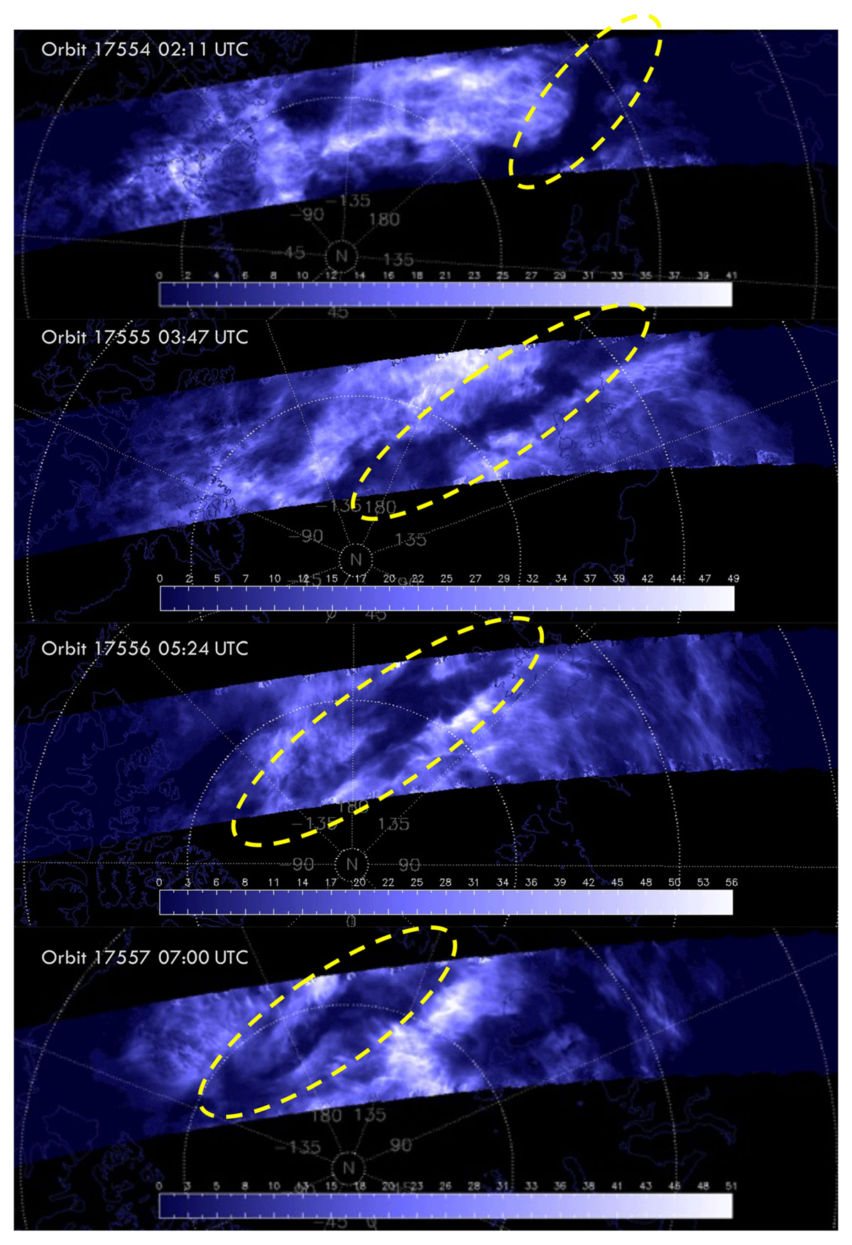
Figure 1
CIPS PMC cloud albedo observations during four consecutive orbits on 16 July 2010. The yellow dashed ovals indicate the dark front-like structure. Note the sharp front edge to the surrounding cloud field in orbit 17556.
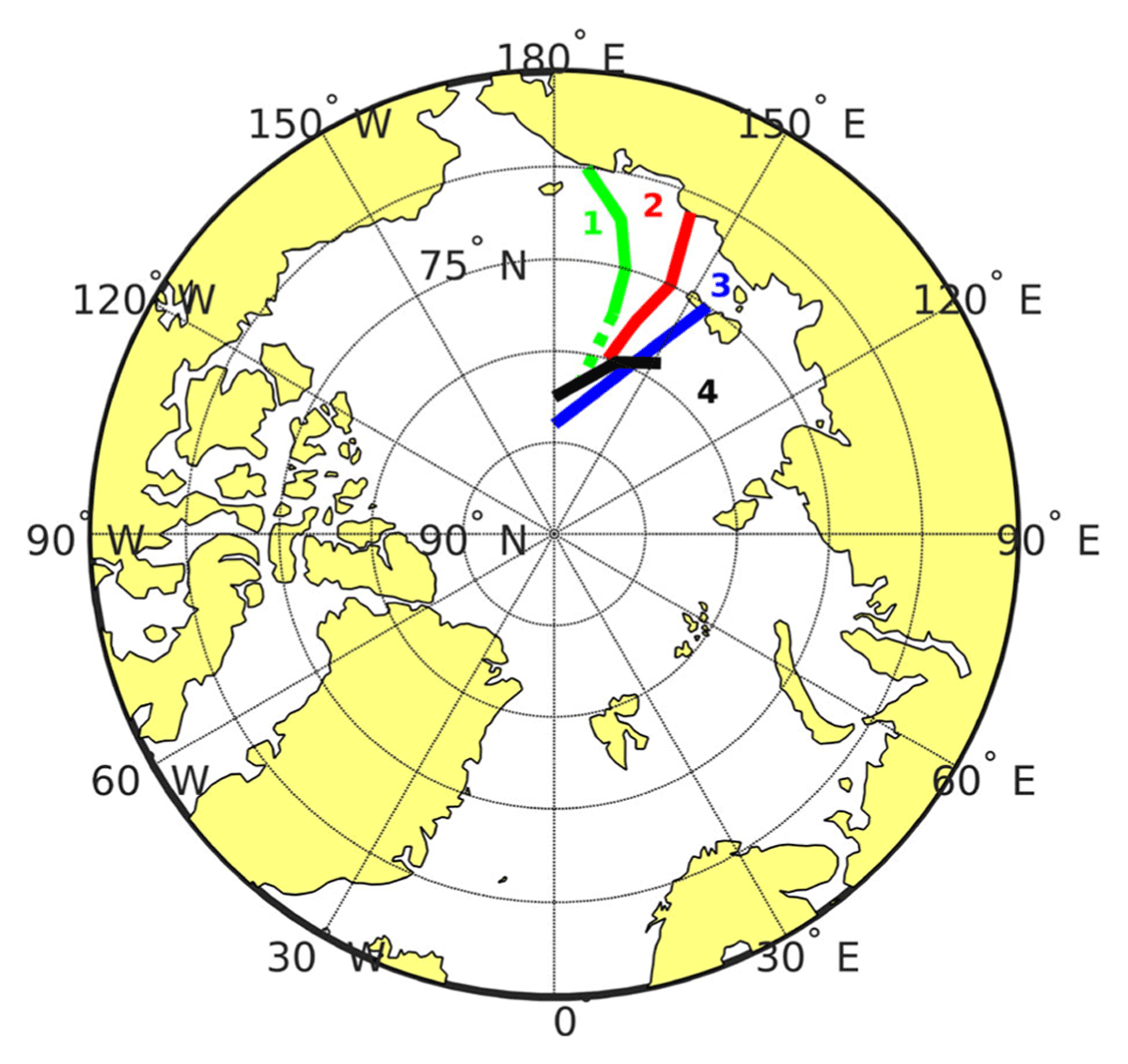
Figure 2
Approximate position of the front structure as observed in CIPS albedo. The numbers refer to the orbits in Figure 1, and the colored lines mark the position of the dark ice free region in each orbit. The view is limited by the CIPS coverage in each orbit swath, and the sketch shows only the part of the structure that is clearly visible. In the first orbit, we use the complementary OSIRIS PMC observations of the front to extend the front position to 78°N (indicated by dotted line).
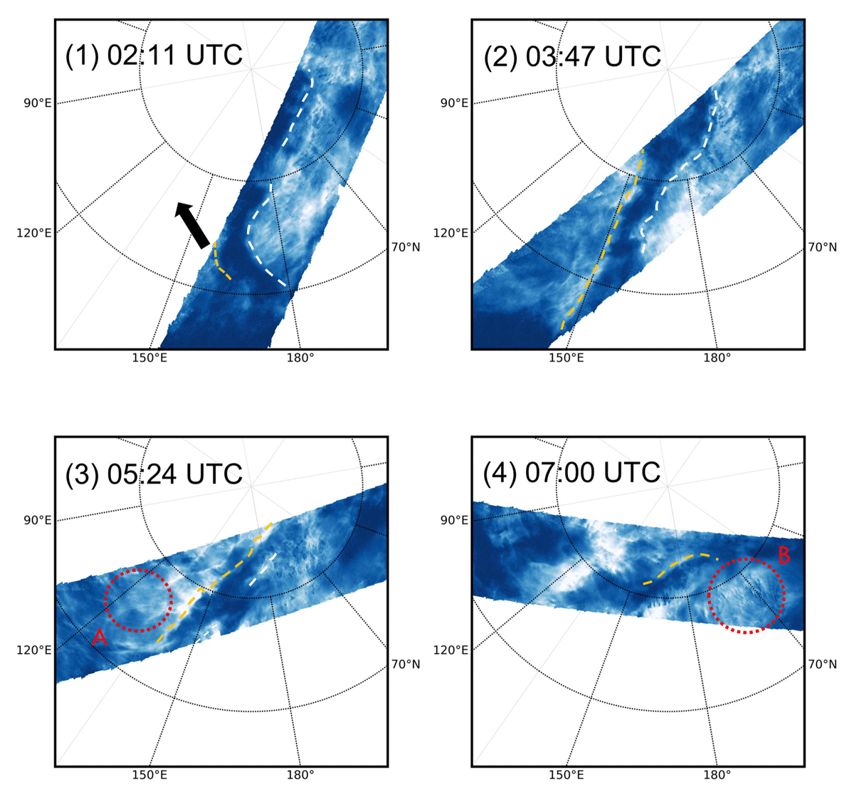
Figure 3
CIPS PMC albedo L2 data projected onto polar map plot centered at 170°E for 4 consecutive orbits showing the progression of the front region and location of regions with small scale waves. The yellow dashed line marks the leading edge of the front, and the white dashed line marks the trailing edge of the front. Red circles (A, B) marks regions of GW activity. The estimated background northwestward wind from tidal climatologies is indicated in top left plot.
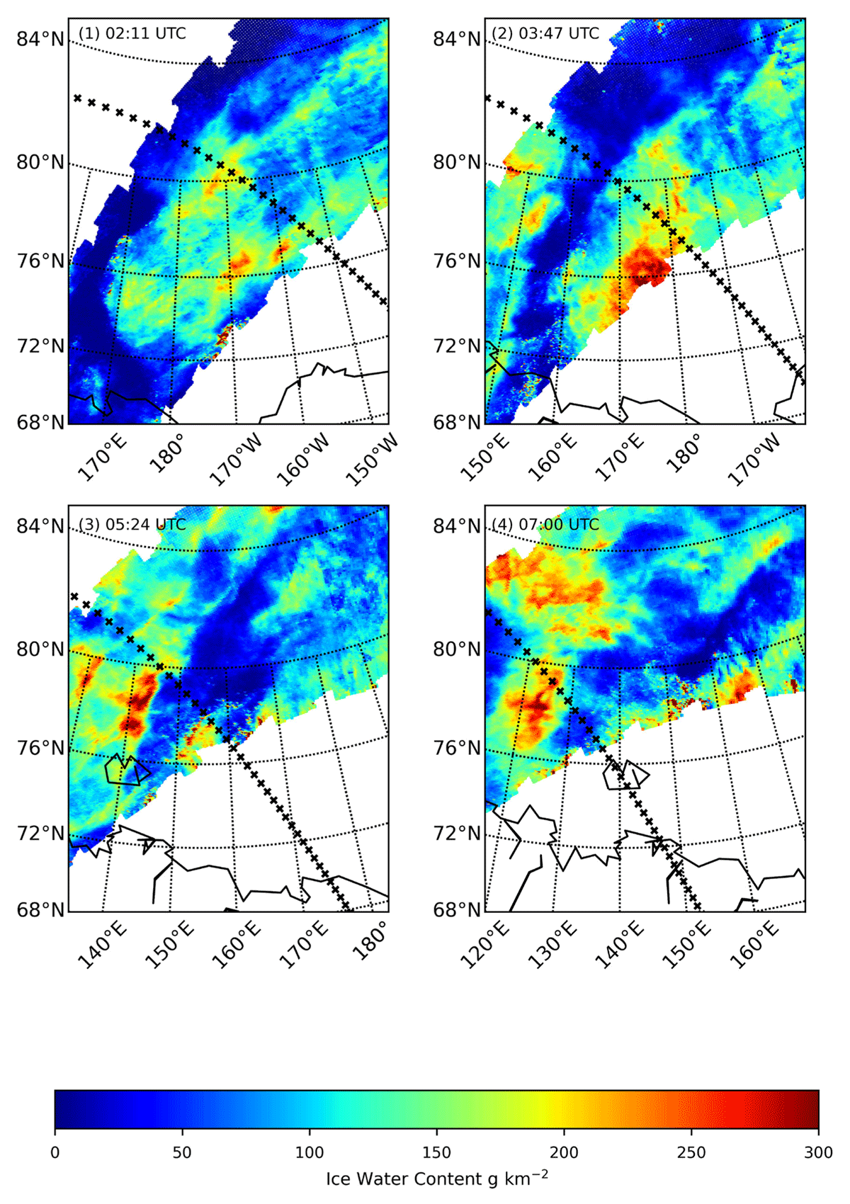
Figure 4
PMC ice water content obtained from CIPS for the four consecutive orbits swaths on 16 July 2010. The orbit start time for CIPS is indicated in each plot. The black crosses mark the position of the coinciding Odin orbit track.
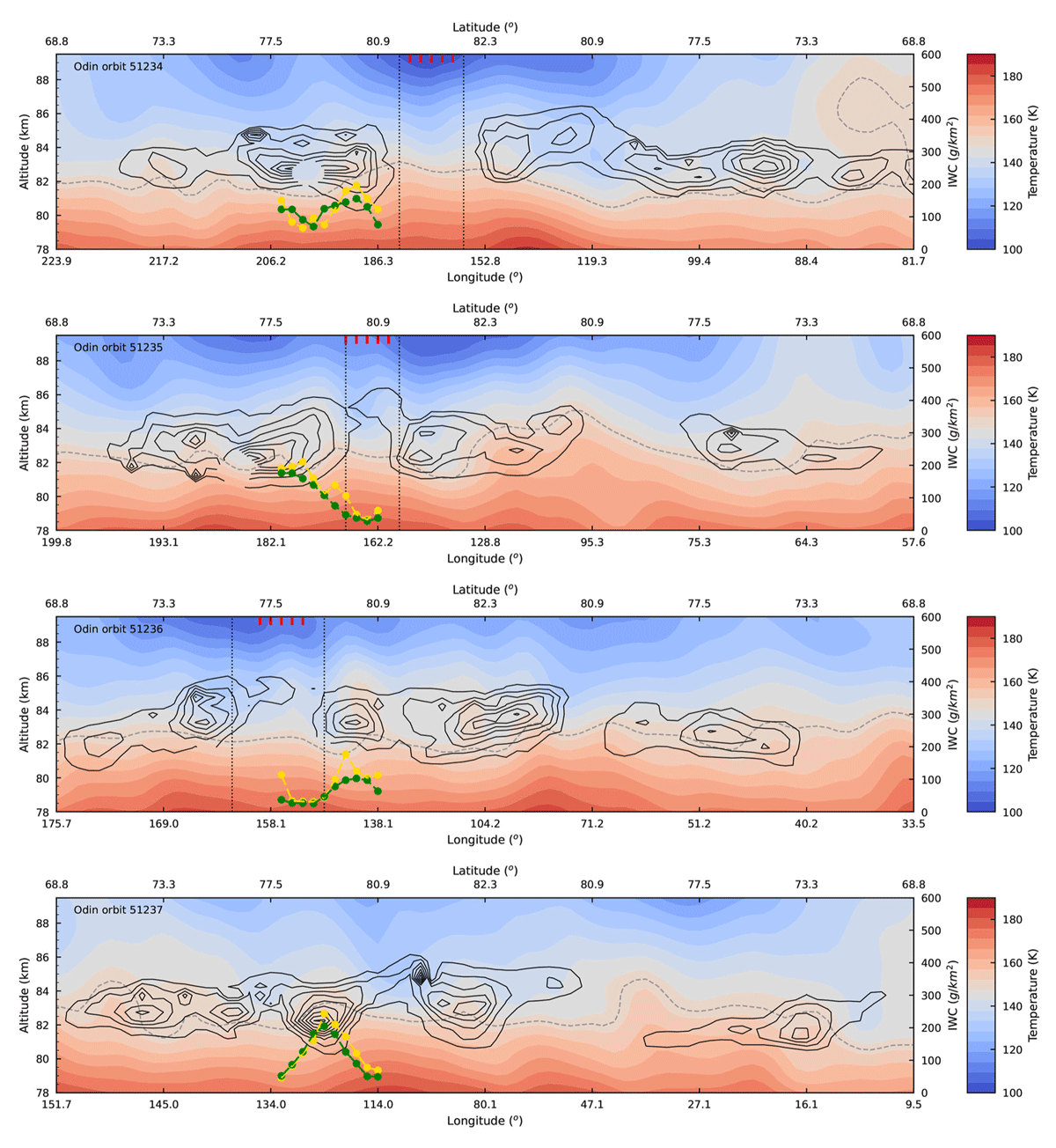
Figure 5
Temperature field from Odin SMR as filled contours combined with simultaneous observations of PMC ice mass density (IMD) from OSIRIS on July 16 2010 for the consecutive orbits 51234–51237. The dashed isoline marks 150 K, where cloud likely sublimates. The black IMD contours correspond to 10 ng/m3. The missing parts of the IMD contours imply missing data. For these retrieval pixels, the microphysical retrieval cannot provide cloud properties using the Ångström relation. CIPS IWC in the common volume is plotted with yellow line and OSIRIS IWC is plotted with green line (right y-axis). Red ticks on upper x-axis denote profiles used in Figure 8.
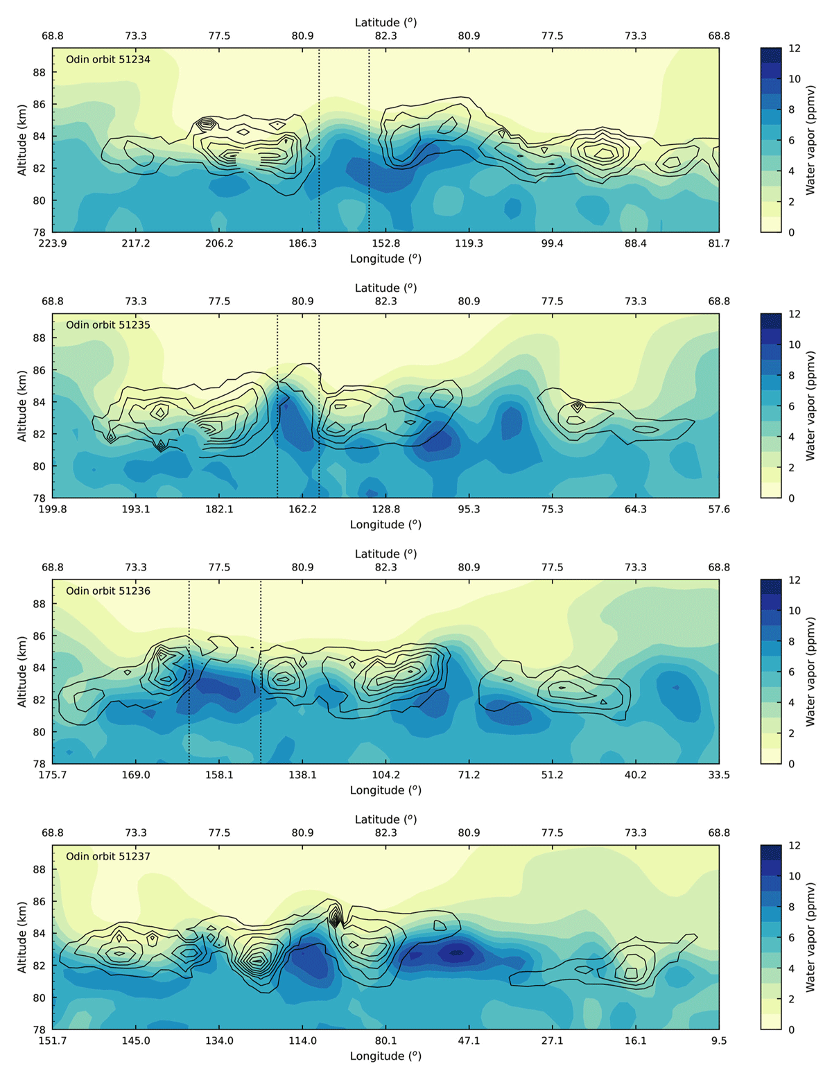
Figure 6
Odin SMR Water Vapor as coloured contours combined with OSIRIS ice mass density as black contours. The dashed lines indicate front (ice free) region as simultaneously observed by CIPS. The missing parts of the IMD contours imply missing data. For these retrieval pixels, the microphysical retrieval cannot provide cloud properties using the Ångström relation.
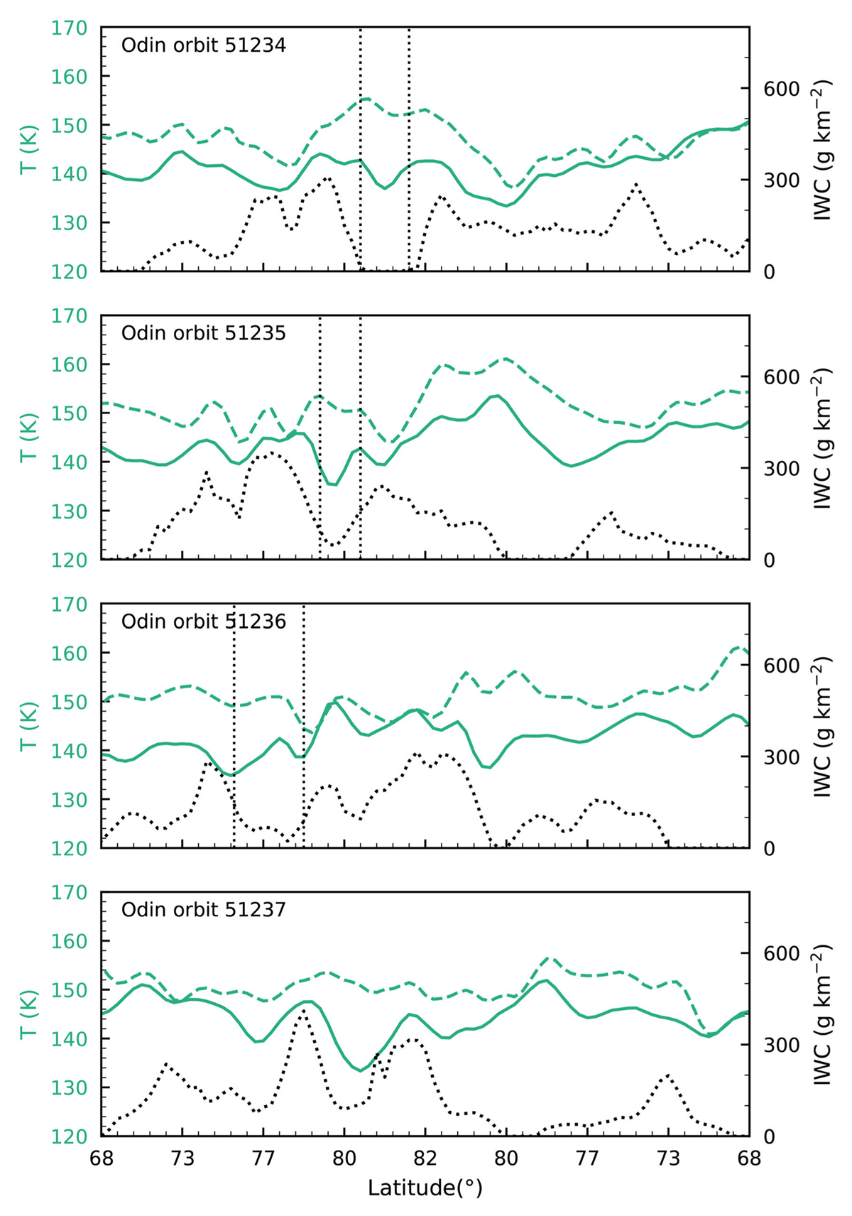
Figure 7
SMR Temperature observations on July 16 shown as transects at constant altitude 84.25 km (dashed line) and 82.25 km (solid line) versus latitude for the four Odin orbits (51234, 51235, 51236, 51237). Common volume observations of OSIRIS ice water content (dotted black line) show the vertically integrated ice mass density. The vertical lines show the edges of the front.
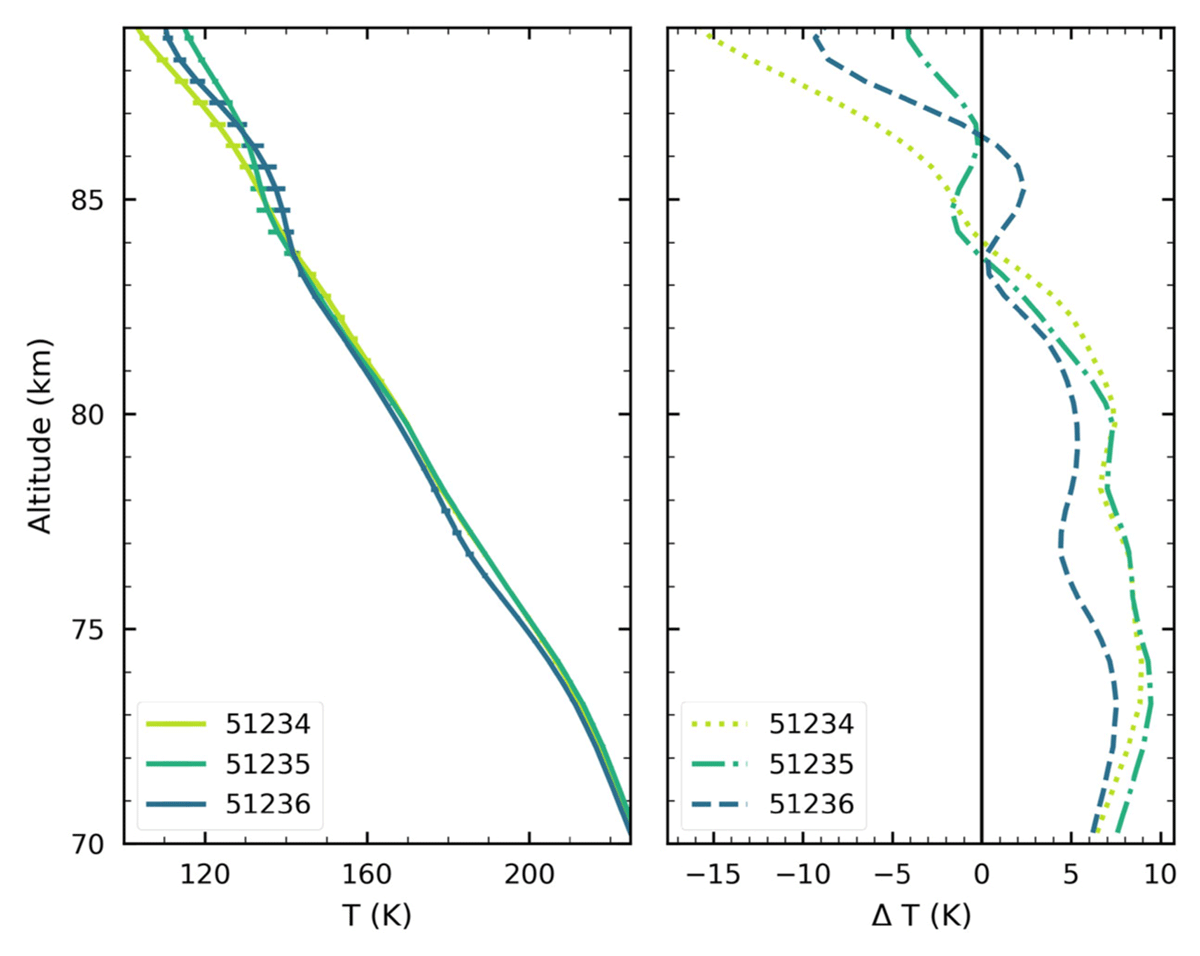
Figure 8
Temperature inside the cloud free region obtained from SMR tomography during the mesospheric front event for the Odin orbits (51234–51236). Left panel shows the temperature profiles where each profile is an average of 5 profiles within the cloud free region. Right panel shows the deviation compared to a 3-day average around the time for the observation for 75°N.
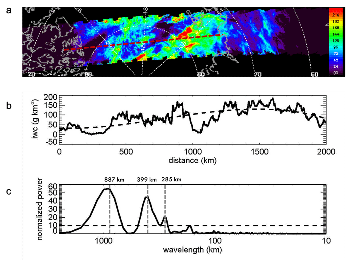
Figure 9
(a) CIPS PMC ice water content for orbit 17556 observed on July 16, 2010. (b) Ice water content along a scan cross the quasi-periodic structures marked by the red dashed line in (a) as a solid line and a polynomial fit (dashed line) to the data to represent the background. (c) Horizontal wavelength against the normalized power spectra of the event. The dashed horizontal line shows the 95 confidence level of the analysis.
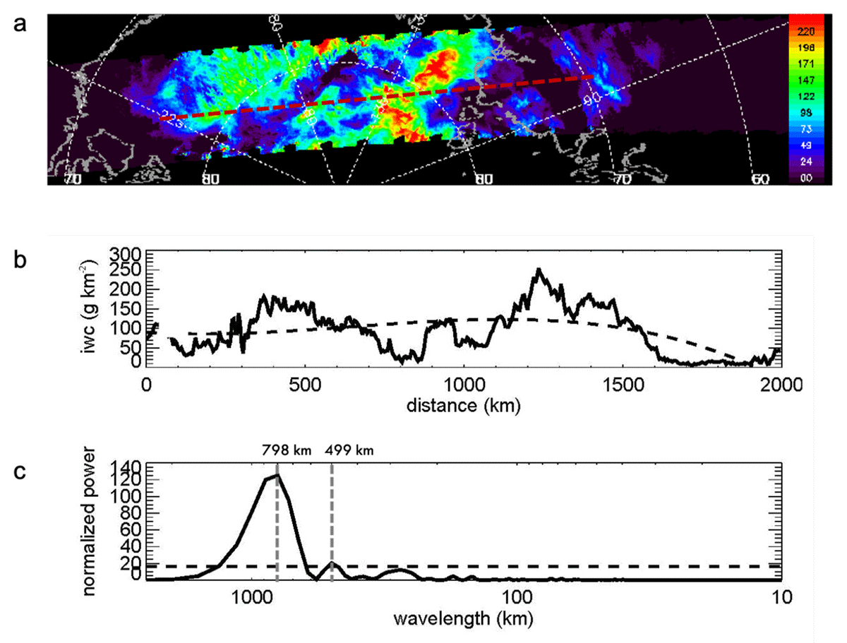
Figure 10
Same as Figure 9 but for CIPS orbit 17557.
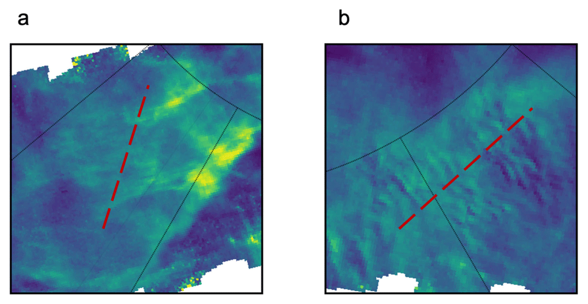
Figure 11
Enlargement of CIPS PMC ice water content for orbit 17556 and 17557 observed on July 16. (a) and (b) are regions marked A and B in Figure 3. Red dashed line marks scan across wave structures.
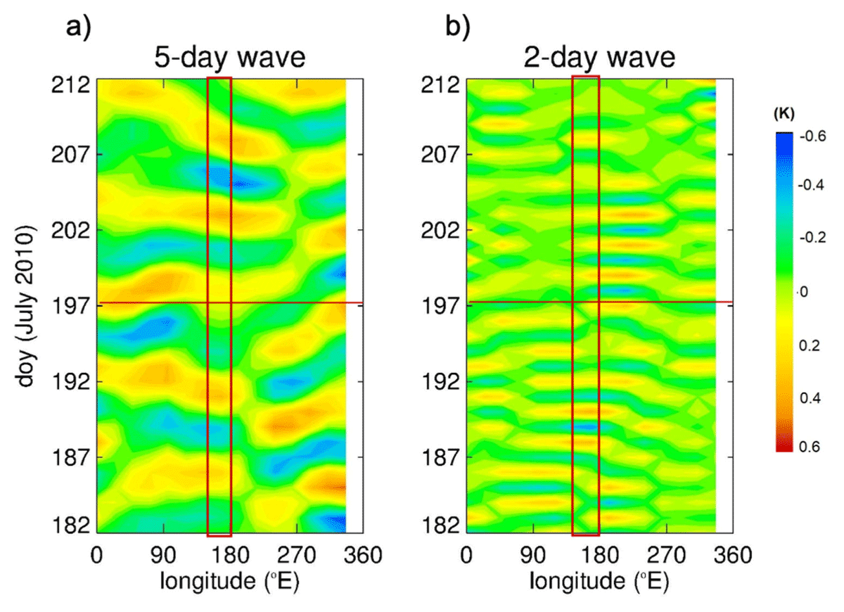
Figure 12
Longitude-time plots of temperature amplitude for the 5-day wave (a) and for the 2-day wave (b) for day of year 182 to 212 2010 from MLS temperature. The red lines denote the occurrence of the mesospheric front.