
Table 1
12 CMIP6 models that provide all diagnostics necessary for this study.
| MODEL ACRONYM | RESOLUTION LAT ×LON | REFERENCE |
|---|---|---|
| CNRM-CM6-1-HR | 360 × 720 | Voldoire et al. (2019) |
| CNRM-ESM2-1 | 128 × 256 | Séférian et al. (2019) |
| EC-Earth3-Veg | 256 × 512 | Döescher et al. (2021) |
| GISS-E2-1-G | 90 × 144 | Miller et al. (2021) |
| INM-CM4-8 | 120 × 180 | Volodin et al. (2018) |
| IPSL-CM6A-LR | 143 × 144 | Boucher et al. (2020) |
| MIROC-ES2L | 64 × 128 | Hajima et al. (2020) |
| MPI-ESM-1-2-HAM | 96 × 192 | Tegen et al. (2019) |
| MPI-ESM1-2-HR | 192 × 384 | Müller et al. (2018) |
| MPI-ESM1-2-LR | 96 × 192 | Mauritsen et al. (2019) |
| MRI-ESM2-0 | 160 × 320 | Yukimoto et al. (2019) |
| UKESM1-0-LL | 144 × 192 | Sellar et al. (2019) |
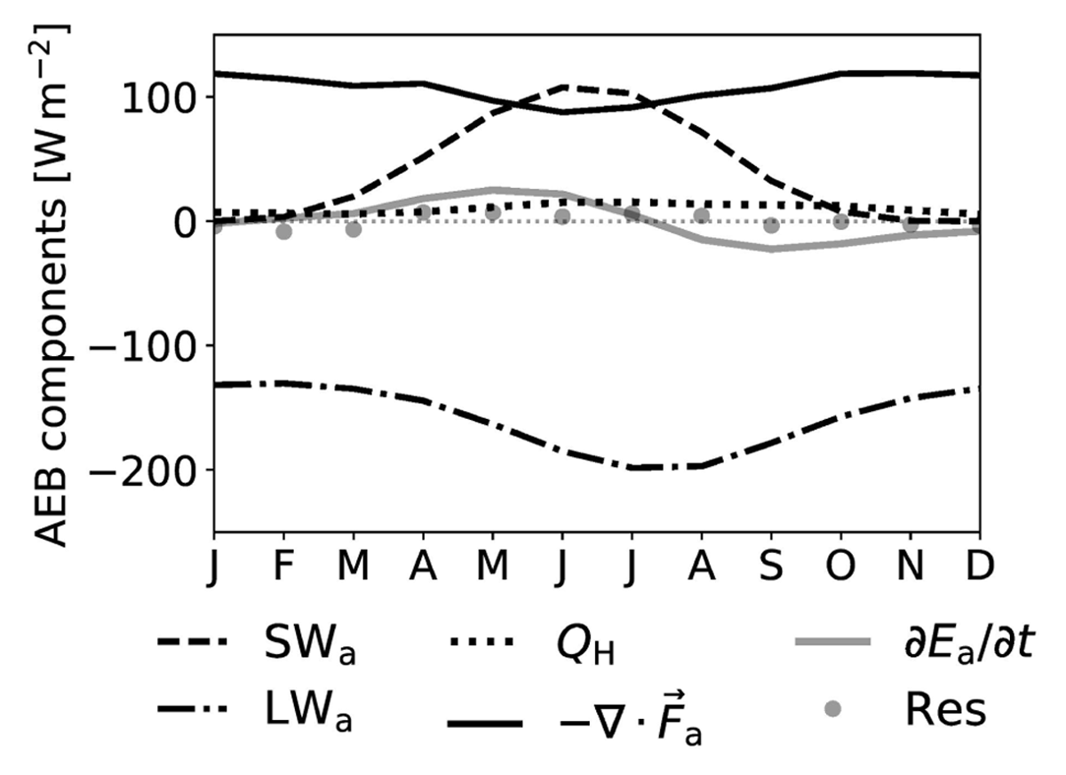
Figure 1
Annual cycle of the pan-Arctic AEB. All values are derived as 30-year climatological averages from piControl of the IPSL-CM6A-LR model. AEB components account for the atmospheric energy storage ∂Ea/∂t, the atmospheric radiation budget (SWa and LWa contributions), the net surface turbulent heat flux (QH = Qh + Qe), and the convergence of atmospheric energy transport –∇ ∙ Fa. The residual is derived by summing up all budget components and substracting the energy storage tendency.
Table 2
Components of the pan-Arctic AEB from the IPSL-CM6A-LR model averaged over spring (MAM), summer (JJA), fall (SON), and winter (DJF), derived from 30-year averages 1970–1999 of piControl. The corresponding annual cycle is presented in Figure 1. Uncertainty intervals are calculated as the inter-annual standard error.
| CHANGES IN ENERGY FLUXES AND STORAGE TENDENCY [W m–2] | |||||||
|---|---|---|---|---|---|---|---|
| SEASON | SWa | LWa | Qh | Qe | –∇∙ Fa | ∂Ea/∂t | RESIDUAL |
| MAM | 52.8 ± 0.1 | –147.4 ± 0.4 | 0.9 ± 0.2 | 7.3 ± 0.2 | 105.5 ± 1.2 | 16.5 ± 0.7 | 2.6 ± 1.0 |
| JJA | 94.0 ± 0.1 | –193.5 ± 0.4 | 4.1 ± 0.1 | 10.7 ± 0.1 | 93.5 ± 0.8 | 4.1 ± 0.3 | 4.7 ± 0.7 |
| SON | 13.5 ± 0.0 | –159.3 ± 0.4 | 1.5 ± 0.2 | 9.9 ± 0.2 | 114.9 ± 1.1 | –17.3 ± 0.5 | –2.2 ± 0.8 |
| DJF | 1.1 ± 0.0 | –132.3 ± 0.6 | –0.8 ± 0.3 | 7.2 ± 0.2 | 116.9 ± 2.1 | –2.4 ± 1.0 | –5.4 ± 1.2 |
| Annual mean | 40.4 ± 0.0 | –158.1 ± 0.3 | 1.4 ± 0.1 | 8.8 ± 0.1 | 107.7 ± 0.7 | 0.2 ± 0.1 | –0.1 ± 0.5 |
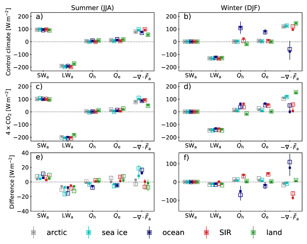
Figure 2
Seasonal components of the Arctic AEB from CMIP6 simulations, with left panels representing summertime, and right panels showing wintertime, respectively. Panels a and b: control model run (piControl), c and d: quadrupled-CO2 climate from 1pctCO2, e and f: the corresponding differences (1pctCO2 minus piControl). The tendency in atmospheric energy storage is negligible, i.e., the AEB components add up to zero. All components are derived as climatological (30-year) averages, and are further categorised into four surface types. From the ensemble of 12 climate models, larger squares indicate the average of six models with higher AA, smaller squares give the model average of six models with weaker AA, respectively. Errors bars indicate the inter-model standard deviation. Note that the scale of changing fluxes in panel e and f is 1:4 for summer vs.winter.
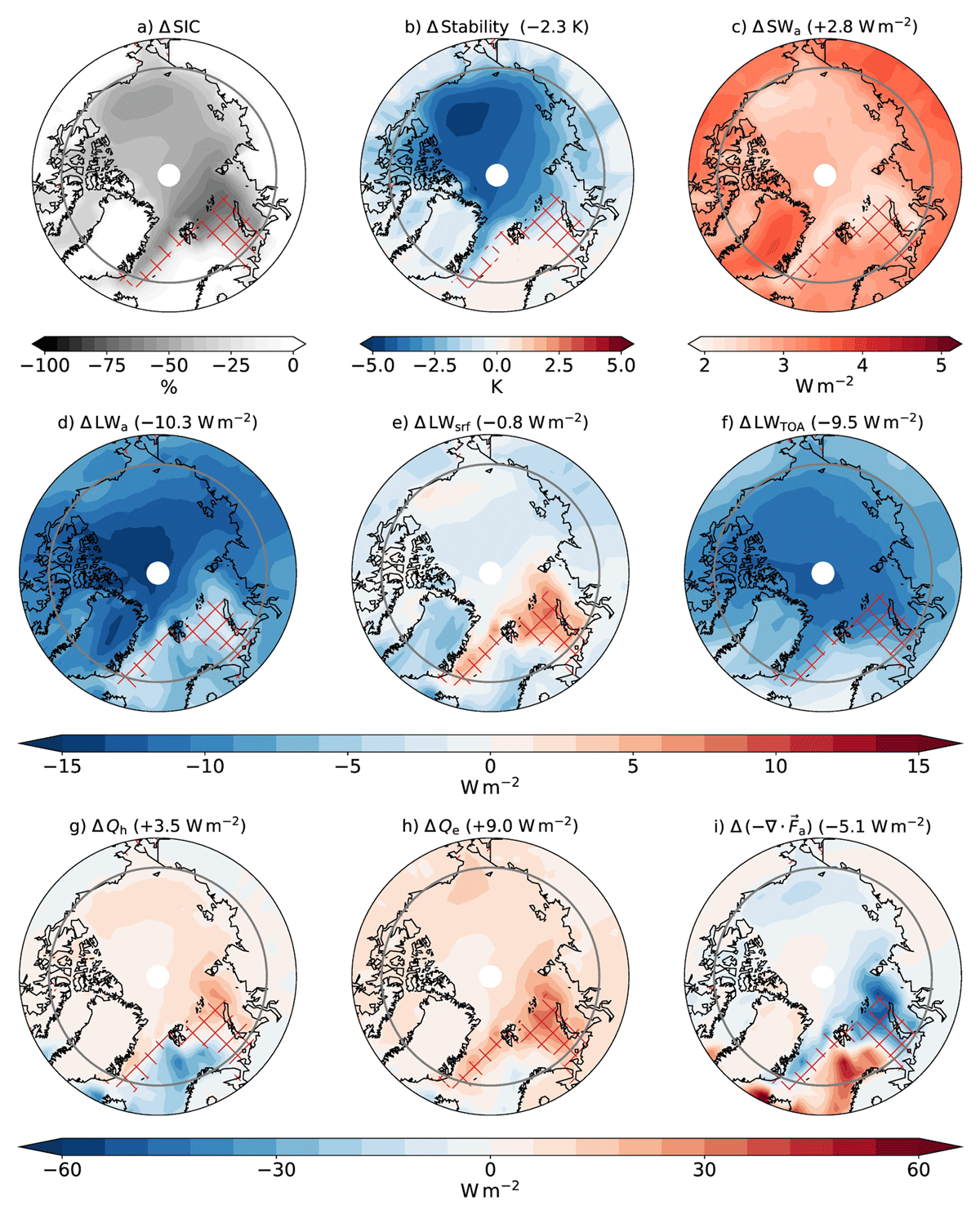
Figure 3
CO2-driven annual differences in the AEB components between the quadrupled-CO2 and control climate from CMIP6 simulations. Changes are further shown for SIC (panel a) and stability (panel b). The LWa term is additionally broken down into net contributions from the surface (panel e), and the TOA (panel f). All components are calculated as 30-year climatological mean, and multi-model averages from 12 CMIP6 models. The 70°N latitude is marked in gray. Pan-Arctic averages are given on top of each panel. Each map shows the distribution of maximum occurrence of the SIR surface type marked by red hatching.
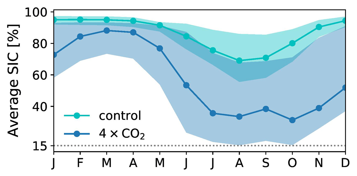
Figure 4
Annual cycle of pan-Arctic SIC averaged over the ice-covered ocean. The annual cycle is given for both the model control simulation and quadrupled-CO2 conditions from CMIP6. The curves show the multi-model average and the shaded areas include data from all 12 climate models.
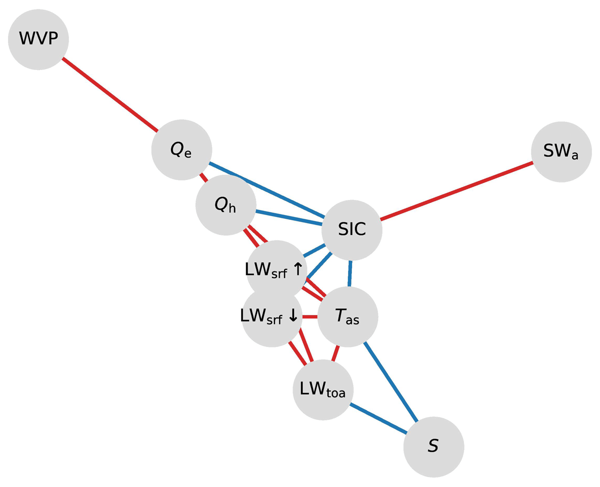
Figure 5
Correlation network plot including all Pearson correlations of annual-mean diagnostics that are significant at the 99% level and above the r threshold of 0.6. The distance of the nodes accounts for the degree of correlation, with smaller distances indicating a stronger correlation. Red (blue) colouring indicates positive (negative) correlations. Spatial correlations are restricted to the sea-ice covered ocean domain, where sea ice does not retreat.