
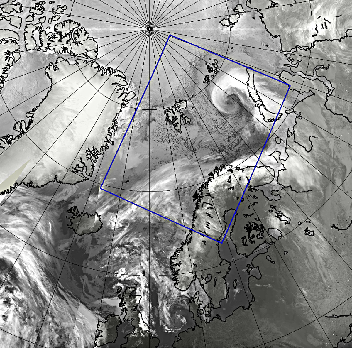
Figure 1
The AROME-Arctic domain shown by the blue rectangle.
Table 1
Case study periods and periods used for SST error estimation.
| DATE | NAME | EVENT | PERIOD FOR ERROR ESTIMATION |
|---|---|---|---|
| 2019-10-29 to 2019-10-31 | PL | Polar low | 2019-10-28 to 2019-11-03 |
| 2020-01-04 to 2020-01-05 | CAO I | Cold air outbreak | 2019-12-30 to 2020-01-05 |
| 2020-02-04 to 2020-02-05 | STR | Storm over northern Norway | 2020-02-03 to 2020-02-09 |
| 2020-03-10 to 2020-03-12 | CAO II | Cold air outbreak | 2020-03-09 to 2020-03-15 |
| ALL | All case studies together |
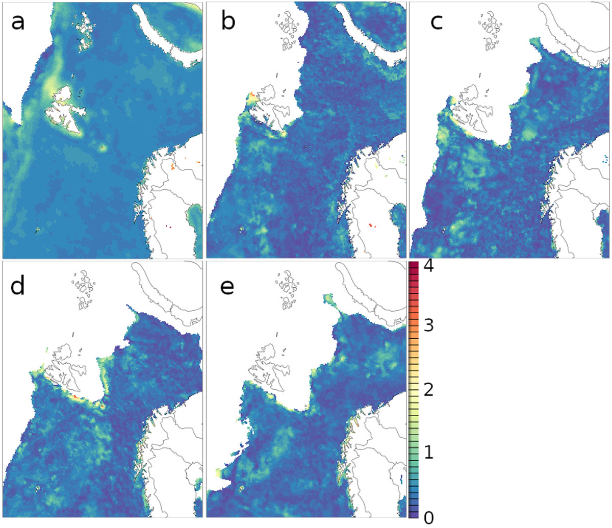
Figure 2
Error estimation fields, ɛ – a) 2018; b) 2019-10-28 to 2019-11-03; c) 2019-12-30 to 2020-01-05; d) 2020-02-03 to 2020-02-09; e) 2020-03-09 to 2020-03-15.
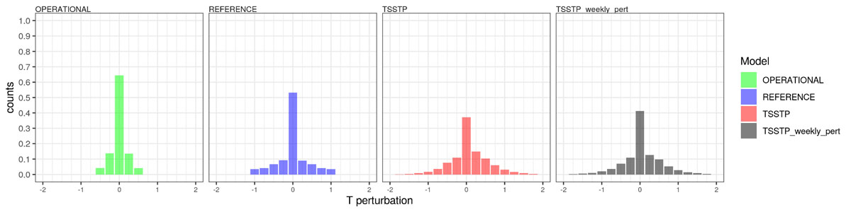
Figure 3
Histograms of perturbations for each experiment.
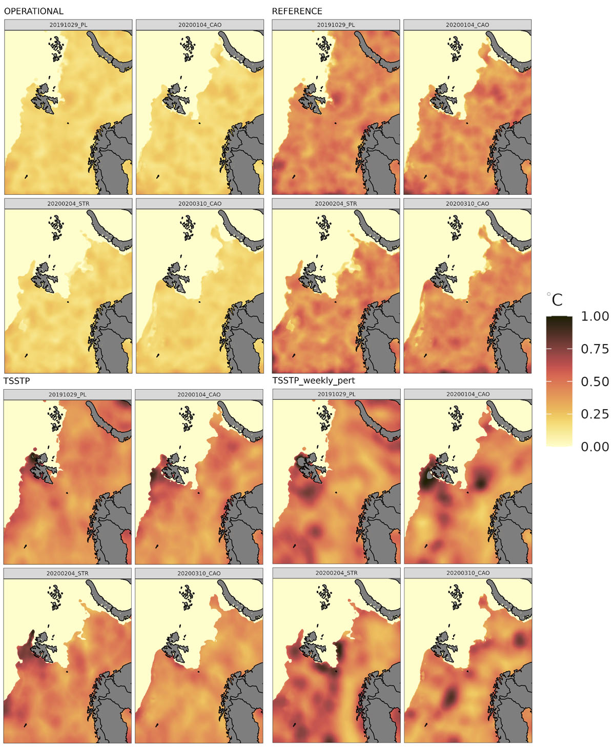
Figure 4
Mean absolute SST perturbations for OPERATIONAL (top left panel), REFERENCE (top right panel), TSSTP (bottom left panel) and TSSTP_weekly_pert (bottom right panel) for each experiment period individually.
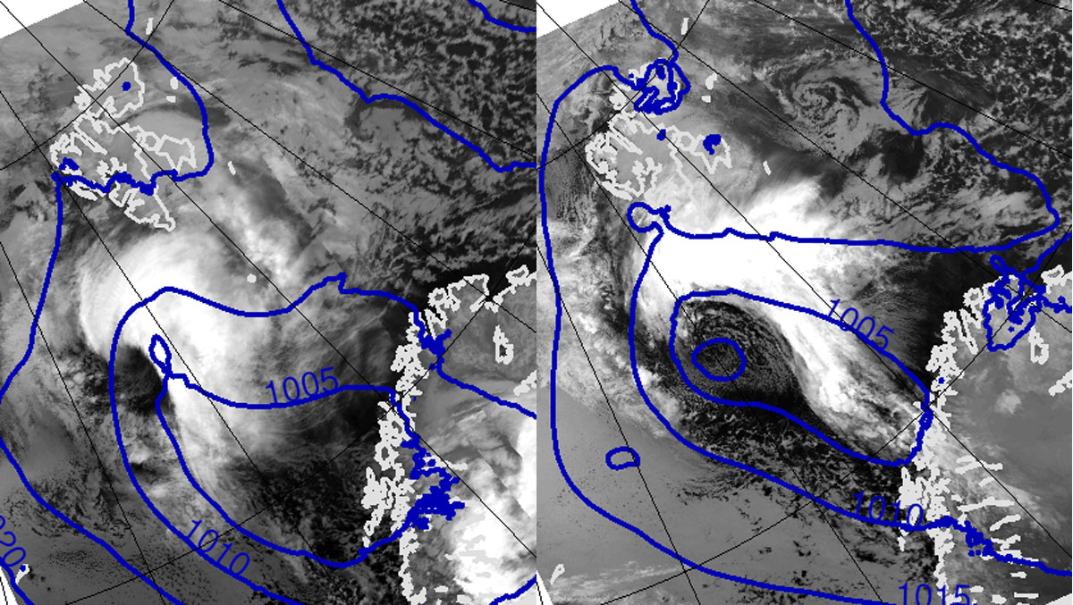
Figure 5
Synoptic situation during PL case study. Satellite image and mean sea level pressure. From left to right: 2019-10-30 21 UTC and 2019-10-31 12 UTC.
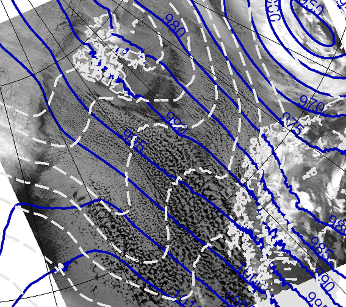
Figure 6
Synoptic situation during the CAO I case study. Satellite image, mean sea level pressure (solid lines) and thickness 500 – 1000 hPa layer (dashed lines). 2020-01-04 12 UTC.
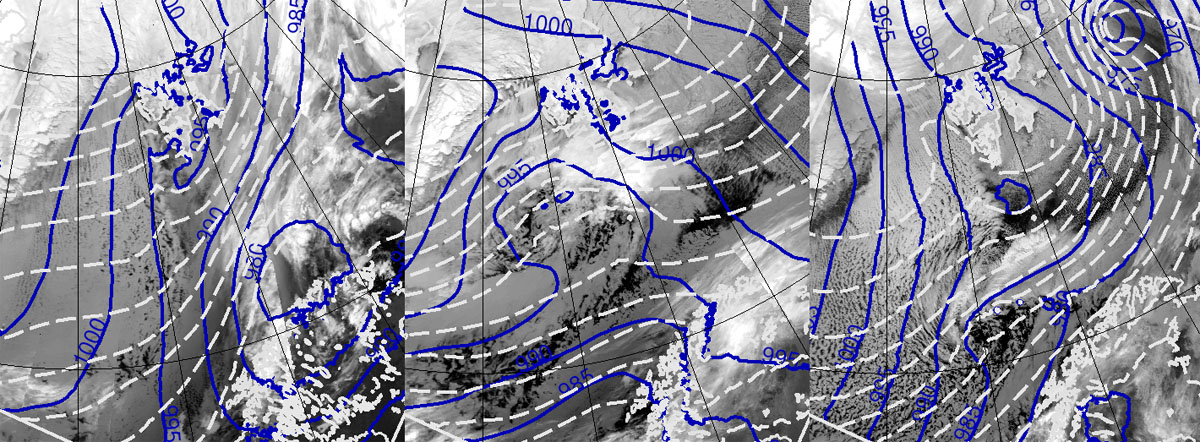
Figure 7
Synoptic situation during the CAO II case study. Satellite image, mean sea level pressure (solid lines) and thickness of the 500 – 1000 hPa layer (dashed lines). From left to right: 2020-03-10 00 UTC, 2020-03-11 06 UTC and 2020-03-12 09 UTC.
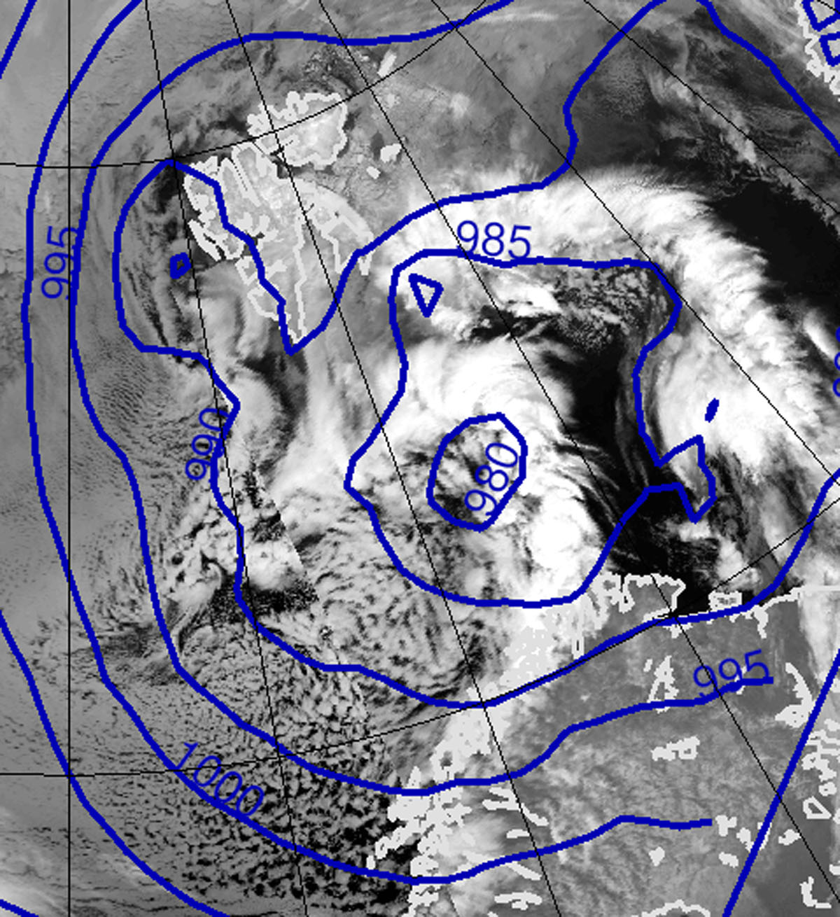
Figure 8
Synoptic situation during the STR case study. Satellite image and mean sea level pressure. 2020-02-05 03 UTC.
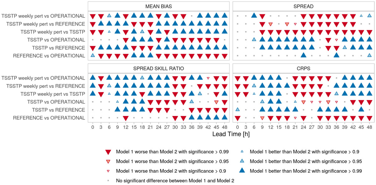
Figure 9
Comparison of the experiments regarding mean sea level pressure.
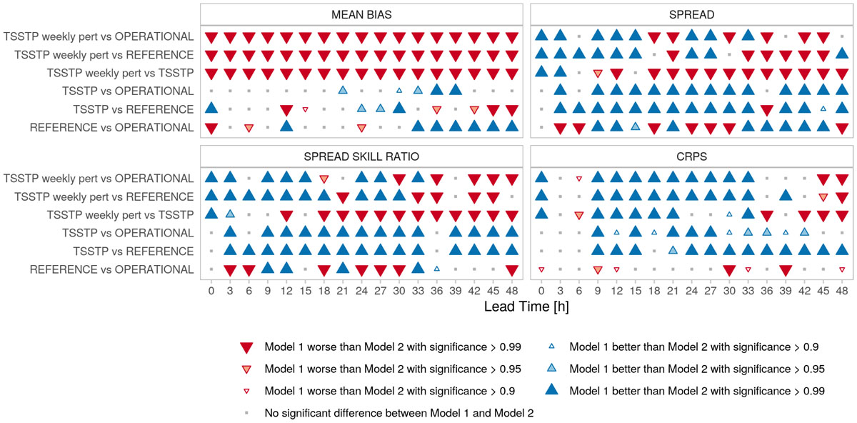
Figure 10
Comparison of the experiments regarding 2 m temperature.
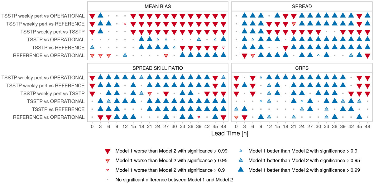
Figure 11
Comparison of the experiments regarding 2 m specific humidity.
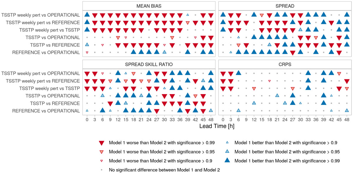
Figure 12
Comparison of the experiments regarding 10 m wind speed.
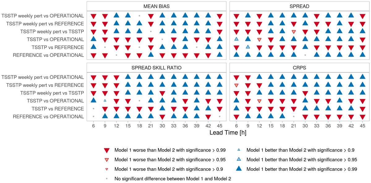
Figure 13
Comparison of the experiments regarding 10 m wind speed based on verification with ASCAT wind data.
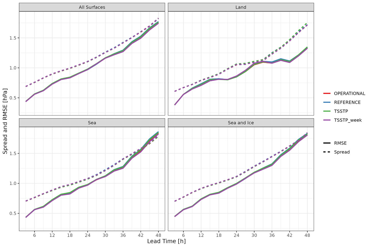
Figure 14
Spread and RMSE for mean sea level pressure.
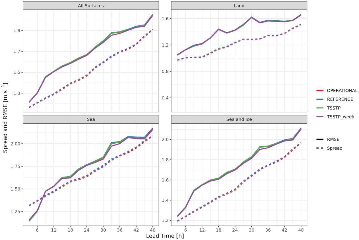
Figure 15
Spread and RMSE for 10 m wind speed.
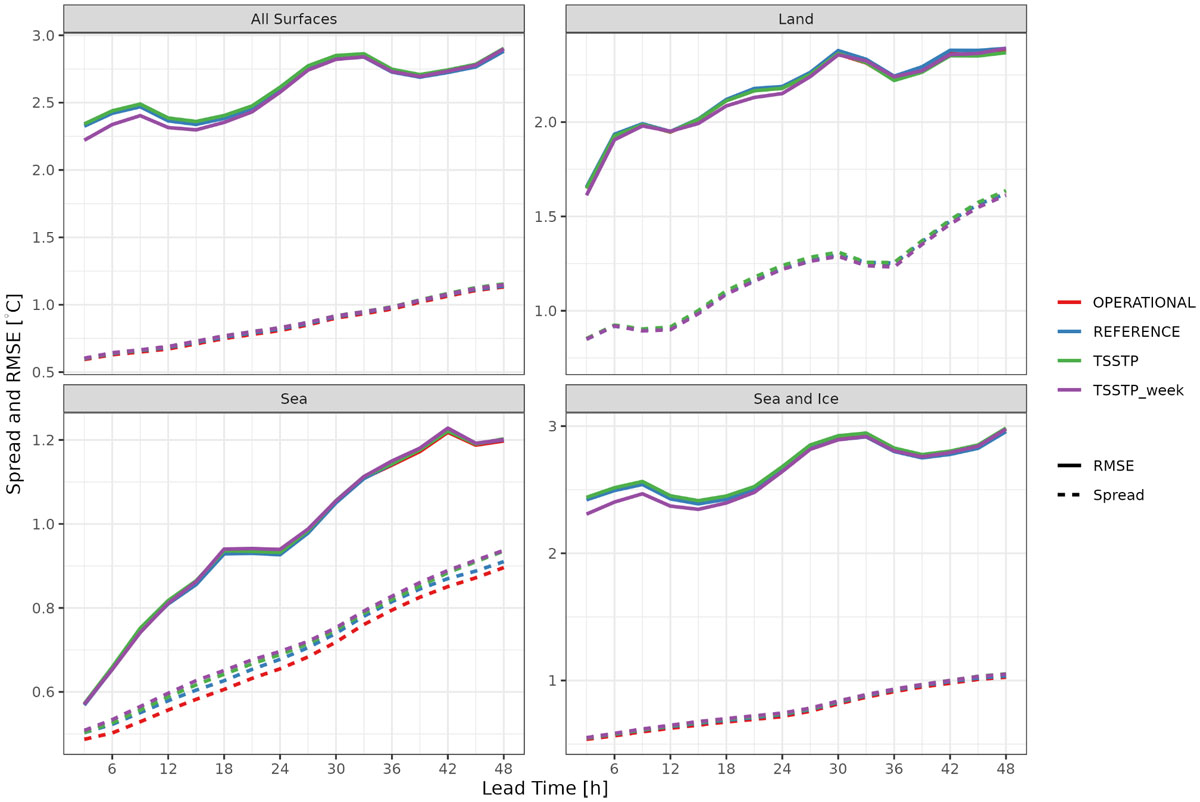
Figure 16
Spread and RMSE for 2 m temperature.
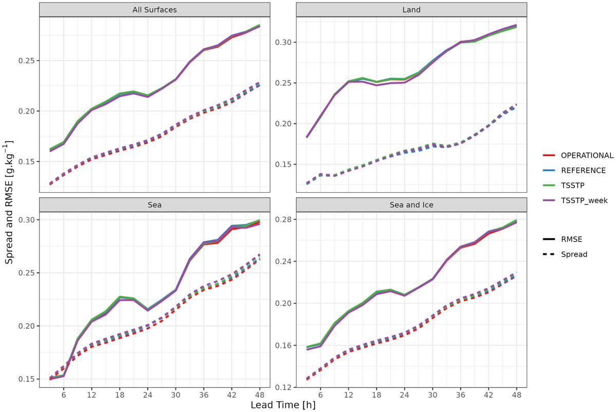
Figure 17
Spread and RMSE for 2 m specific humidity.
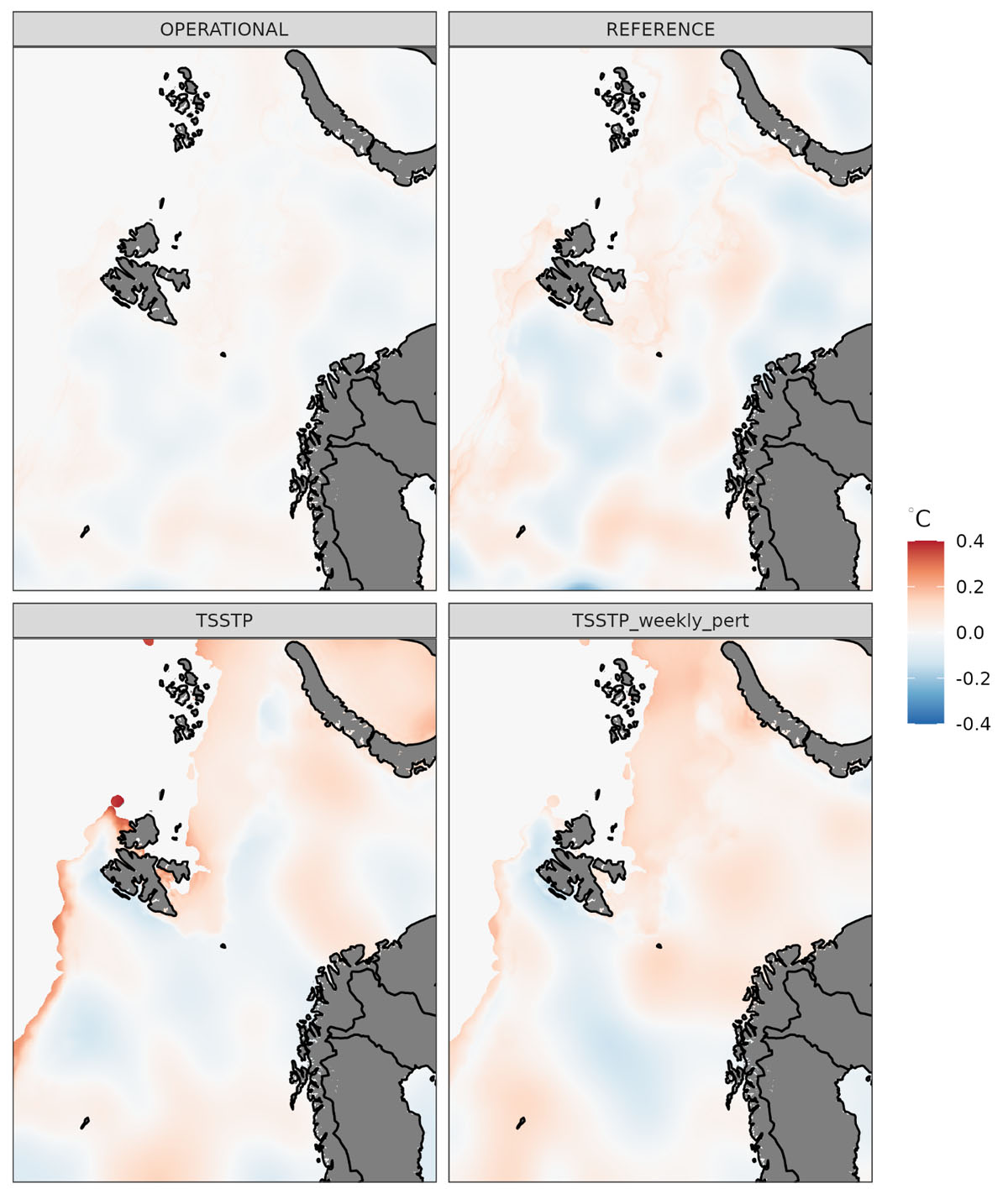
Figure 18
Mean SST perturbations for each of the perturbation methods averaged over all forecasts.