
1 Introduction
Human activity, such as oil and gas exploration, fishing and maritime cargo transport, as well as tourism have all increased dramatically over recent years in the Arctic and that trend is likely to continue as sea ice coverage continues to lessen. While oil and gas exploration in the Arctic is a controversial topic where political as well as environmental factors could play a decisive role in its future, for maritime transport, for example, the Northern Sea Route opened to international shipping in 2010 and cuts transit time between northwest Europe and northeast Asia by 14–20 days compared to the Suez route. Although transiting traffic has been lower than expected due to economic and political factors as well as the availability of suitable container ships, destination voyages have increased in the years to 2019 (Gunnarsson and Moe, 2021). Moreover, shipping traffic as a whole has increased markedly in the Arctic Ocean in recent years with tens of thousands of ships operating there in 2014, the majority in the Norwegian and Barents Seas (Eguíluz et al., 2016). In terms of tourism, the Arctic archipelago Svalbard, for example, has experienced an approximate doubling in tourist numbers in the 10 years from 2010 to 2019 accompanied by a shift from seasonal to year-round tourism (Hovelsrud et al., 2021).
This increased activity in the Arctic means that the provision of accurate and reliable weather forecasts is becoming increasingly important. However, numerical weather prediction (NWP) models for high latitudes generally show lower forecast capability compared to other regions (Jung et al., 2016). The challenges are many – NWP models have typically been developed to maximise forecast accuracy over mid-latitude regions; a relative scarcity of in situ observations make it difficult to provide accurate initial states for the forecasts and to determine comprehensive verification statistics; and the physics and dynamics of high latitude extreme weather systems are less well understood. Furthermore, the challenging environment of the region with less infrastructure and difficult conditions for search and rescue means that forecast misses can have dramatic consequences both for local communities and those operating in the region.
Since 2015, the Norwegian Meteorological Institute (MET Norway) has provided high resolution, short range (up to 66 hours lead time) operational weather forecasts for an area that includes the coast of northern Scandinavia, parts of the Norwegian-, Greenland- and Barents Seas, and the Svalbard archipelago (Figure 1) using the AROME-Arctic model. AROME-Arctic is a non-hydrostatic convection permitting deterministic NWP model with a grid length of 2.5 km in the horizontal and 65 terrain following vertical levels (Køltzow et al., 2019; Müller et al., 2017a). AROME-Arctic is a specific implementation of the HARMONIE-AROME configuration of the ALADIN-HIRLAM numerical weather prediction system (Bengtsson et al., 2017), with a setup that closely follows developments made with the AROME-MetCoOp operational model (Müller et al., 2017b), which runs operationally for a domain that covers the Nordic countries.
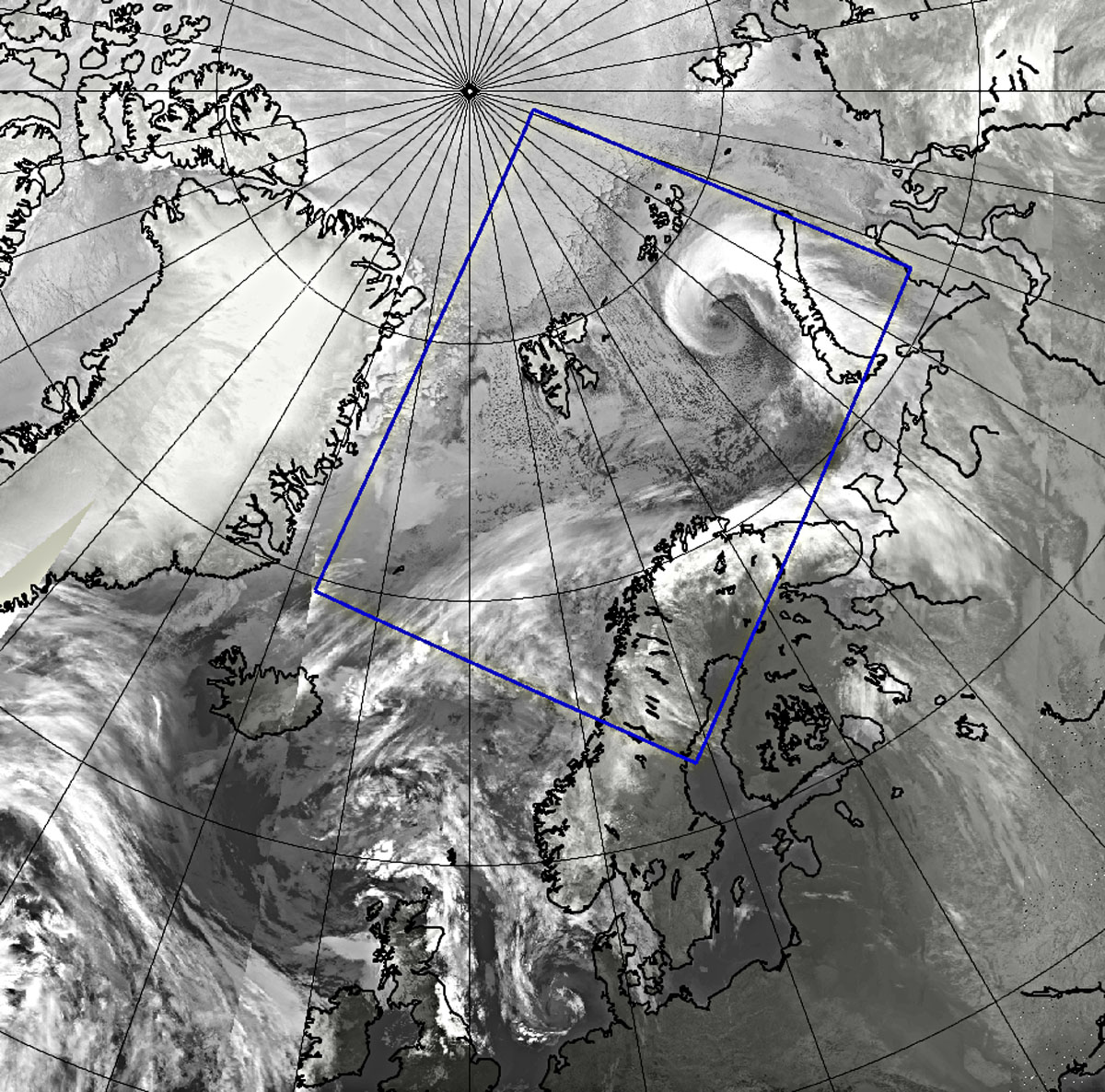
Figure 1
The AROME-Arctic domain shown by the blue rectangle.
The relative scarcity of observations in the Arctic region means that it is to be expected that there is considerable uncertainty in the forecasts that AROME-Arctic produces. It is therefore important to model that uncertainty so that users and stakeholders can make better informed decisions in a risk based environment where the consequences of weather hazards can be extremely damaging, both economically and in the potential for severe injury or loss of life. The development of ensemble prediction systems (EPS) has enabled uncertainties that stem from many parts of the NWP model to be estimated (Lewis, 2005). Considerable work has been done on the development of global EPSs by estimating uncertainties in the initial conditions (e.g. Buizza and Palmer, 1995; Toth and Kalnay, 1993), uncertainties in observations (e.g. Isaksen et al., 2010) and uncertainties in model physics parameterizations (e.g. Ollinaho et al., 2017; Palmer et al., 2009). As computational power has increased the development of convection permitting limited area ensembles has become possible whereby uncertainty estimation also includes boundary and initial condition uncertainty emanating from the host model (e.g. Bouttier et al., 2016; Frogner et al., 2019; Hagelin et al., 2017; Wang et al., 2011).
The AROME-Arctic domain is approximately 85% ocean (although more than half of that could have some, or complete, sea ice cover depending on the time of year) so it would be reasonable to expect that energy fluxes between the ocean surface and the atmosphere play an important role in the evolution of weather parameters, particularly in the atmospheric boundary layer. Sea surface temperature (SST) is an important component in the computation of the fluxes of sensible and latent heat between the ocean and the atmosphere so inaccuracies in the SST at the lower boundary of the NWP model could have significant impacts on the forecasts. Indeed Donlon et al. (2012) showed that Operational Sea Surface Temperature and Sea Ice (OSTIA) product, which is used to provide SST in AROME-Arctic, exhibits an average root mean square error (RMSE) over the Arctic Ocean of 0.72 K when compared with satellite observations and 0.46 K when compared with in situ observations for a period covering 1 January 2007 to 31 December 2010.
A number of studies have been done to determine the impact of including uncertainty estimates for SST in EPSs. Tennant and Beare (2014) used both global and regional implementations of the MOGREPS model to investigate the impact of perturbing SST fields with the spatial scaling properties of perturbations derived from fast Fourier transforms (FFT) of daily differences in SST, further scaled by the mean daily difference in SST for the month. They found that this led to an increased spread for 2 m temperature of ~0.5–1 K over the European Arctic ocean. Where observations were available over land they found negligible impact on the RMSE in terms of global average. However, they did note that in some regions increases in spread of 2 m temperature over the ocean were compensated by decreases in spread over land. Lavaysse et al. (2013) perturbed SST in the Canadian regional ensemble prediction system using spatially smoothed random fields with a decorrelation length scale of 500–1000 km. They found a similar impact on 2 m temperature over the ocean to Tennant and Beare (2014), but also noted increases in spread for precipitation and 10 m wind speed in precipitating areas. Bouttier et al. (2016) and Frogner et al. (2019) use a similar stochastic method to perturb for their convection permitting EPSs with decorrelation length scales of ~400 and ~150 km respectively, though they do not discuss the impact of the SST perturbations acting alone.
The aforementioned studies make the case for perturbing SST in EPSs, but what is not clear is to what extent the location and magnitude of SST perturbations matter. In this article we aim to address that question, specifically for high impact weather events over the AROME-Arctic domain. A comparison is made between purely stochastic, but spatially correlated SST perturbations and SST perturbations that are designed to target the locations where the uncertainty is largest, for a number of high impact weather events using an EPS implementation of the AROME-Arctic NWP model.
Following this introduction, the article is organised as follows: Section 2 describes the EPS implementation of the AROME-Arctic model, the methods used to generate the SST perturbations, the high impact weather events and the verification metrics used. Section 3 presents the results of the experiments and a discussion of those results and conclusions follow in Section 4.
2 Methods
2.1 Model Description
The model used for this study is based on the AROME-Arctic model (Køltzow et al., 2019; Müller et al., 2017b); the operational implementation of the Harmonie-AROME model (Bengtsson et al., 2017) for the Arctic region around Norway used at MET Norway. The model is set up similar to the Harmonie EPS system (Frogner et al., 2019) to provide ensemble forecasts. It runs with a 2.5 km horizontal grid length and 65 terrain following vertical hybrid layers. The domain the experiments were run on covers parts of the northern Scandinavian mainland and European Arctic and is shown in Figure 1.
The control member of the ensemble used three dimensional variational (3DVAR; Brousseau et al., 2011) to assimilate upper air observations from radiosondes and satellites with three hour cycling, and optimal interpolation to assimilate observations of 2 m temperature and 2 m humidity (Giard and Bazile, 2000). The data assimilation used three-hour cycling and the control member was spun up for 10 days prior to each experiment. In addition to the data assimilation the model included a blending of large spatial scales from the global model providing boundary conditions in order to obtain a more accurate first guess.
The Integrated Forecasting System High Resolution (IFS HRES) from the European Center for Medium-Range Weather Forecasts (ECMWF) was used to perturb the lateral boundary and initial conditions for forecasts initialised at 00 UTC. Perturbations were generated using the scaled lagged average forecast (SLAF) approach (Ebisuzaki and Kalnay, 1991; Kalnay, 2019), where differences between lagged forecasts from IFSENS with the same validity time are added to or subtracted from the control member of the model. The perturbations were scaled using the total energy norm (Keller et al., 2008) to ensure that each perturbation has roughly the same impact on the forecast. The model was run with 10 perturbed members in addition to the control member.
Surface processes were modelled using SURFEX (Masson et al., 2013), which included a sea ice model that uses a simple thermodynamic scheme (Batrak et al., 2018). For all experiments surface parameters were perturbed at the forecast initialization time following Frogner et al. (2019). These parameters include the following physiographic variables: vegetation index, vegetation heat coefficient, leaf area index, land albedo and land roughness length; as well as the prognostic variables: soil temperature, soil moisture and snow depth. In addition surface fluxes over the ocean are perturbed with the same pattern at each time step to simulate the perturbation of roughness length of the sea. The perturbations were applied multiplicatively except for the soil temperature, which was applied additively. The perturbation patterns were generated by applying a recursive filter to a normalised field of stochastic noise sampled from a uniform distribution until a correlation length scale of ~150 km was achieved. The normalisation is scaled according to a prescribed standard deviation for each of the perturbed parameters. The seed for the stochastic noise generation is derived from the forecast start date.
2.2 SST Perturbations
We wish to compare SST perturbations that are randomly located with those with locations targeted towards regions where the uncertainty is thought to be greatest. For the randomly located SST perturbations we followed the method for the other surface perturbations described above. Following Frogner et al. (2019) a standard deviation of 0.25 K was used and the perturbations were applied additively. Additionally, the perturbation fields were clipped to have minima and maxima of twice the standard deviation. We refer to these experiments as OPERATIONAL since they use the same settings as operational implementations of HARMONIE-AROME EPS.
For the SST perturbations targeted towards regions where the uncertainty is thought to be greatest, a method based on nonparametric noise generation described in Seed et al. (2013) and Pulkkinen et al. (2019) is used. This method is similar to that of Tennant and Beare (2014) in that the power spectrum of an error field is used to determine the spatial scales of the perturbations and a further field that estimates the location and magnitude of the errors is used to scale the perturbations. We refer to this method as targeted SST perturbations (TSSTP) and describe its implementation in detail below.
TSSTP requires an estimate of the error, ɛ, of the initial SST field to derive the spatial correlations from, as well as an SST scaling field, s to derive the magnitude of the SST perturbations for the domain of interest. The generation method consists of the following steps:
Generation of a white noise field, w.
Fast Fourier Transformation of the white noise field w and the SST error estimate, ɛ.
Filtering of the fourier transform of the white noise field, F(w), with the modulus of the fourier transform of the error estimate, |F(ɛ)|, to obtain a perturbation field, F(p), with the spatial correlation structure of the error estimate.
Inverse FFT of the perturbation field, F(p), to transform it from Fourier space to physical space, p.
Normalisation of the perturbation field, p, to a mean of zero and standard deviation of one.
Scaling of the normalised perturbation field by multiplication with a scaling field, s, to obtain the scaled perturbation field.
Addition of the scaled perturbation field, s, to the SST field of the NWP model.
The SST error field, ɛ, was estimated by comparing SST data from the ECMWF IFS HRES operational analysis to the Multi-scale Ultra-high Resolution Sea Surface Temperature Analysis (MUR). Note that the SST from ECMWF IFSHRES is OSTIA data interpolated to the model grid.
The ECMWF HRES operational model is run four times a day with analysis times at 00, 06, 12 and 18 UTC. These data were further interpolated to a global 0.1 x 0.1 degree grid from the IFSHRES grid. The MUR dataset provides global and daily SST data derived from a range of satellites with microwave and infrared sensors with a spatial resolution of 0.01 degrees. The dataset spans 1 June 2002 to the present. The MUR dataset represented the best proxy of the high resolution SST patterns and thus errors in the IFSHRES SST data.
MUR SST and sea ice concentration (SIC) data were cropped and projected to match the extent, resolution and projection of the IFS HRES data. Then the difference of IFS HRES SST to MUR SST was calculated for each grid point. Grid points over landmasses or grid points with a sea ice concentration (SIC) greater than zero in either IFS HRES or MUR were excluded.
The error estimation field, ɛ, was derived by calculating the mean absolute differences for the week covering the experiment periods as described in Table 1. The experiments based on these datasets are called TSSTP_weekly_pert in the following. A second error estimation field was calculated from a dataset spanning the period from 1.1.2018 to 31.12.2018, using the same method as described above, to test the impact of the underlying estimation fields on the perturbation generation and consequently the model. These experiments are labelled TSSTP. The error estimation field, ɛ, was reprojected to fit the model projection and resolution in a final step. The resulting fields are displayed in Figure 2.
Table 1
Case study periods and periods used for SST error estimation.
| DATE | NAME | EVENT | PERIOD FOR ERROR ESTIMATION |
|---|---|---|---|
| 2019-10-29 to 2019-10-31 | PL | Polar low | 2019-10-28 to 2019-11-03 |
| 2020-01-04 to 2020-01-05 | CAO I | Cold air outbreak | 2019-12-30 to 2020-01-05 |
| 2020-02-04 to 2020-02-05 | STR | Storm over northern Norway | 2020-02-03 to 2020-02-09 |
| 2020-03-10 to 2020-03-12 | CAO II | Cold air outbreak | 2020-03-09 to 2020-03-15 |
| ALL | All case studies together |
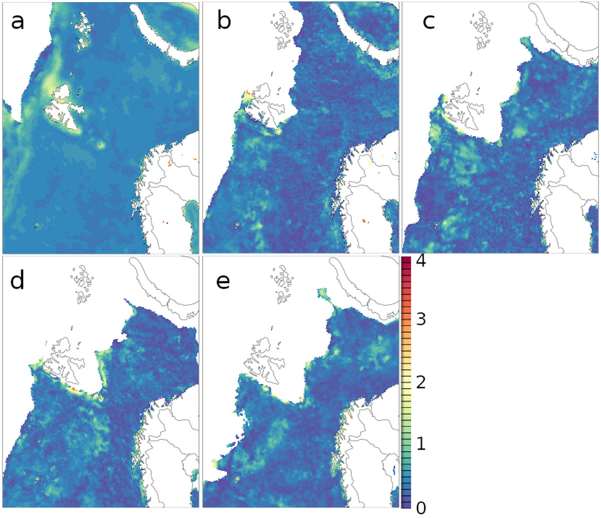
Figure 2
Error estimation fields, ɛ – a) 2018; b) 2019-10-28 to 2019-11-03; c) 2019-12-30 to 2020-01-05; d) 2020-02-03 to 2020-02-09; e) 2020-03-09 to 2020-03-15.
For simplicity we choose to use the error estimation field, ɛ, as the scaling field, s, in this study. However, this is not a general requirement and both ɛ and s can be different fields.
Following an analysis of the perturbations generated for the OPERATIONAL and TSSTP experiments (not shown) it was found that the L1 norm of the perturbations was smaller for OPERATIONAL (~0.3 K) than for TSSTP or TSSTP_weekly_pert (~0.5 K). A further experiment was done with the same setup as OPERATIONAL, but with the standard deviation of the SST perturbations inflated to 0.55 K, such that the L1 norm of the perturbations was roughly equal to that for TSSTP or TSSTP_weekly_pert. We refer to this experiment as REFERENCE as it provides a fairer reference against which to assess the TSSTP and TSSTP_weekly_pert experiments.
2.3 Periods Used for Case Studies
The impacts of the different SST perturbations were studied in four case studies. The periods of the case studies are listed in Table 1. The model was run with lead times up to 48 hours from 00 UTC for each day in the case study periods for the OPERATIONAL, TSSTP, TSSTP_weekly_pert and REFERENCE experiments. The case studies were mostly chosen for meteorological situations in which SST plays an important role. These include a Polar low case and two cold air outbreak cases. A fourth case consisted of the passage of a storm low over northern Norway, which is not particularly tied to SST, but should give an indication of the EPS performance for a typical situation of high impact weather.
2.4 Verification Methodology
The verification and comparison of the SST perturbation methods was done against point observations using the harp software package developed for the HIRLAM and ALADIN consortia (https://harphub.github.io/harp). Forecasts were verified against observations from SYNOP stations for the surface parameters mean sea level temperature, 2 m temperature, 2 m specific humidity and 10 m wind speed. The AROME-Arctic domain covers for the most part ocean and the SYNOP stations are mainly on the Scandinavian mainland and on the Arctic islands, which limits their representativeness. The verification of 10-m wind speed was therefore repeated with Advanced Scatterometer (ASCAT) data with a resolution of 12.5 km. Additionally, the root mean square error (RMSE) and spread was calculated for the whole domain by verifying against operational analyses from the AROME-Arctic model (Müller et al, 2017a).
The verification metrics used in this study are: mean bias as a measure of the average forecast error; spread as a measure of the difference between the ensemble members, represented by the square root of the mean variance of the ensemble members; spread-skill-ratio as the ratio of ensemble spread to the root mean square error the value should be approximately one for a well calibrated ensemble system; and continuous ranked probability score (CRPS) as a measure of the difference between the forecast and observed cumulative distribution function and the general quality of the ensemble.
The statistical significance of the differences between the TSSTP, TSSTP_weekly_pert, OPERATIONAL and REFERENCE experiments with regards to the different scores was determined by Kolmogorov-Smirnov testing on a 1000 replicate bootstrap sample. Scores were computed independently for each experiment and parameter at each lead time from the pool of forecast/observation data. Samples were then drawn randomly with replacement from the computed scores. This was done separately for the TSSTP, TSSTP_weekly_pert, OPERATIONAL and REFERENCE experiments. Pools with fewer than 10 items were ignored. A Kolmogorov – Smirnov test was then used to determine if the samples of the various experiments came from different distributions. The null hypothesis was tested for 1%, 5% and 10% significance levels. The mean of the sampled scores was used to determine the quality of the experiments relative to each other. An experiment was considered to be better than a reference experiment if it had a mean bias or CRPS closer to zero, and if it had a larger spread compared to the reference experiment. The spread skill ratio should ideally approach one. Therefore an experiment was considered better if the distance of its spread skill ratio was closer to one compared to a reference experiment.
3 Results
3.1 Perturbations Comparison and synoptic situation
Histograms of the SST perturbations generated for each experiment were constructed using data from the initial SST for each perturbed ensemble member (Figure 3). Approximately half of the perturbations lie in a range between –0.125 to 0.125 degrees C for each of the methods. The methods for OPERATIONAL and REFERENCE limited the magnitude of the maximum and minimum perturbations, which is apparent in a sharp cut on both ends of the histograms, while there is no limit to the magnitude of perturbations in TSSTP and TSSTP_weekly_pert. The limit for perturbations in OPERATIONAL was smaller resulting in a larger number of perturbations being in the range between –0.375 and 0.375 degrees C compared with REFERENCE, TSSTP and TSSTP_weekly_pert. Both REFERENCE, TSSTP and TSSTP_weekly_pert are very similar for perturbations up to +/– 0.875 degrees C.
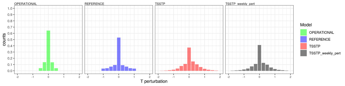
Figure 3
Histograms of perturbations for each experiment.
Figure 4 shows a direct comparison of the mean magnitudes of the perturbations for the various experiments and case study periods. Since each experiment uses the same seed to generate the random numbers, the initial white noise field is the same for each experiment. Both OPERATIONAL and REFERENCE show rather homogeneous perturbation fields since the locations of the perturbations are fully governed by the initial white noise field. In fact the only difference between OPERATIONAL and REFERENCE is the perturbation amplitude due to the inflated standard deviation used in the generation of the perturbations for REFERENCE. Both TSSTP and TSSTP_weekly_pert show perturbations with comparable magnitude as REFERENCE, as intended by the design of the REFERENCE perturbations, but do not display the same homogeneity since the scaling field has a large influence on the locations of the strongest perturbations. This is especially apparent for the perturbation fields of TSSTP_weekly_pert. The error estimation field, used in the perturbation generation and scaling, of TSSTP, is based on the mean absolute error of a longer period when compared to TSSTP_weekly_pert. This results in a smoothing of the perturbation fields for TSSTP. TSSTP shows areas with stronger perturbations mainly west of Svalbard, while TSSTP_weekly_pert shows additional strong perturbations over the whole domain as these represent the uncertainties in the SST in the week preceding each of the weather events.
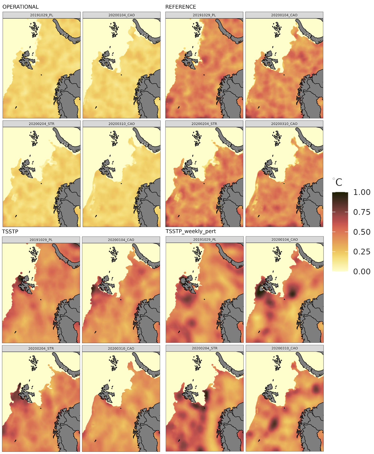
Figure 4
Mean absolute SST perturbations for OPERATIONAL (top left panel), REFERENCE (top right panel), TSSTP (bottom left panel) and TSSTP_weekly_pert (bottom right panel) for each experiment period individually.
Satellite cloud observations and synoptic analyses for the case study period for the polar low case from 29–31 October 2019 showed the development of a polar low southwest of Svalbard, which moved eastwards eventually hitting the coast of northern Norway (Figure 5). The polar low developed in the wake of a low pressure system that moved from Greenland to the Norwegian mainland during 29 October 2019 and the first half of 30 October 2019. TSSTP and especially TSSTP_weekly_pert show the largest perturbations in the area of the developing polar low.
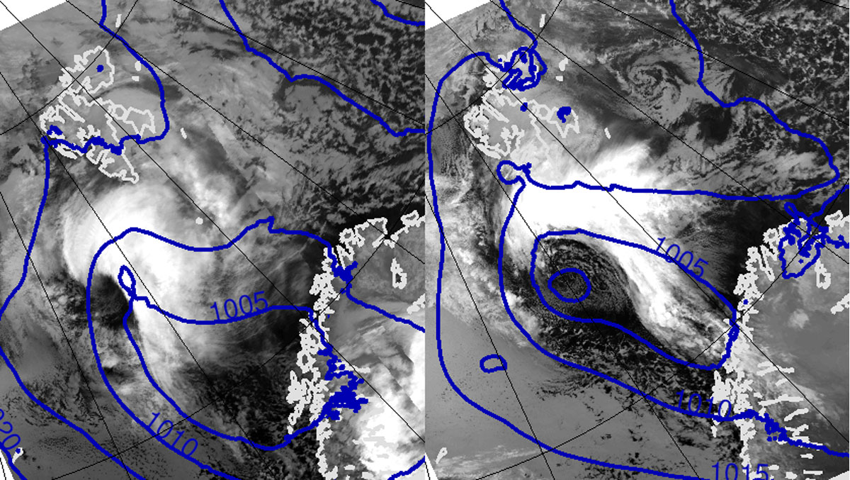
Figure 5
Synoptic situation during PL case study. Satellite image and mean sea level pressure. From left to right: 2019-10-30 21 UTC and 2019-10-31 12 UTC.
The two case study periods covering cold air outbreaks were from 4 January 2020 (CAO I, Figure 6) and from 10–14 March 2020 (CAO II, Figure 7). In both cases the cold air outbreak developed after the passage of a low pressure system south of Svalbard. In both cases cold air masses were transported from the polar region west of Svalbard towards the Norwegian coast, leading to the development of snow showers. For the COA I case, both TSSTP and TSSTP_weekly_pert show the largest perturbations west of Svalbard, the region of the cold air outbreak. The perturbations were not as large for both TSSTP and TSSTP_weekly_pert in the CAO II case. TSSTP shows a rather homogeneous field, while TSSTP_weekly_pert displays the largest perturbations further south of Svalbard.
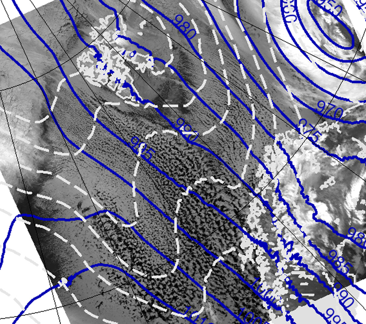
Figure 6
Synoptic situation during the CAO I case study. Satellite image, mean sea level pressure (solid lines) and thickness 500 – 1000 hPa layer (dashed lines). 2020-01-04 12 UTC.
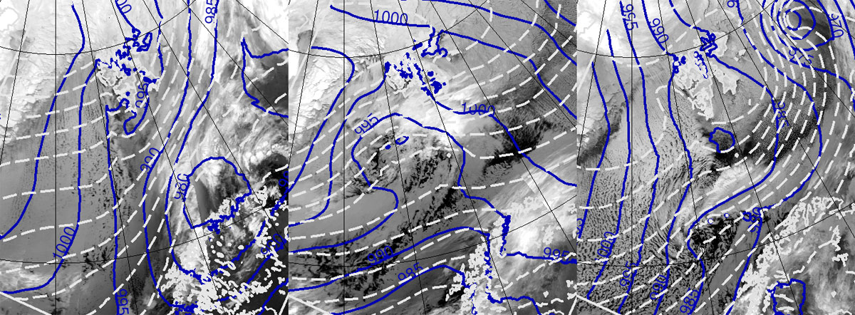
Figure 7
Synoptic situation during the CAO II case study. Satellite image, mean sea level pressure (solid lines) and thickness of the 500 – 1000 hPa layer (dashed lines). From left to right: 2020-03-10 00 UTC, 2020-03-11 06 UTC and 2020-03-12 09 UTC.
The period from 4–5 February 2020 (STR) showed the development of a low pressure system over the Barents Sea (Figure 8), which led to strong winds and snow showers over large areas along the northern Norwegian coast, caused by cold air being transported from the north over the Norwegian sea and towards the Norwegian mainland. TSSTP shows the largest perturbations west of Svalbard and in the area east of Greenland, while TSSTP_weekly_pert shows large perturbations south and southwest of Svalbard, and along the ice-edge east of Svalbard.
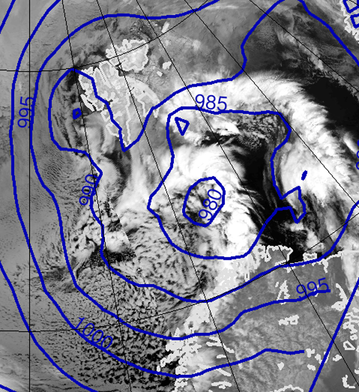
Figure 8
Synoptic situation during the STR case study. Satellite image and mean sea level pressure. 2020-02-05 03 UTC.
3.2 Comparison of perturbations methods based on SYNOP observations
The results of the comparison of the various experiments regarding mean sea level pressure is displayed in Figure 9. The results are mixed for the mean bias. REFERENCE and TSSTP show in general a worse mean bias compared to OPERATIONAL, while TSSTP shows a better mean bias compared to REFERENCE. TSSTP_weekly_pert seems to improve mean bias in comparison to all of the other experiments.
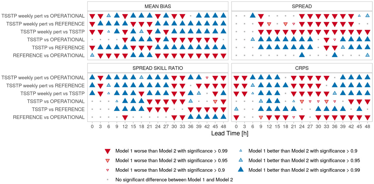
Figure 9
Comparison of the experiments regarding mean sea level pressure.
There is no significant difference in spread between REFERENCE and OPERATIONAL. TSSTP however seems to improve spread, while TSSTP_weekly_pert reduces spread when compared to all other experiments. There are only a few significant differences between TSSTP_weekly_pert and OPERATIONAL or REFERENCE for day one of the forecast.
Both TSSTP_weekly_pert and TSSTP improve the spread skill ratio during the first 27 and 21 hours, respectively, and predominantly show a worse spread skill ratio thereafter. There is only little significant differences between REFERENCE and OPERATIONAL. REFERENCE shows a better spread skill ratio from hour 36.
The CRPS of REFERENCE is worse than that of OPERATIONAL. TSSTP shows a better CRSP when compared to REFERENCE, and less significant differences and mainly a worse CRPS when compared to OPERATIONAL. TSSTP_weekly_pert shows a periodic change between improvement and degradation compared to all other experiments, where improvement occurs mainly during daytime and degradation mainly during night hours.
The results of the comparison regarding 2 m temperature are shown in Figure 10. There is only little significant difference in mean bias between OPERATIONAL, REFERENCE and TSSTP, apart from REFERENCE showing a better mean bias compared to OPERATIONAL from hour 33. TSSTP_weekly_pert shows a worse mean bias compared to all other experiments for the entire forecast period.
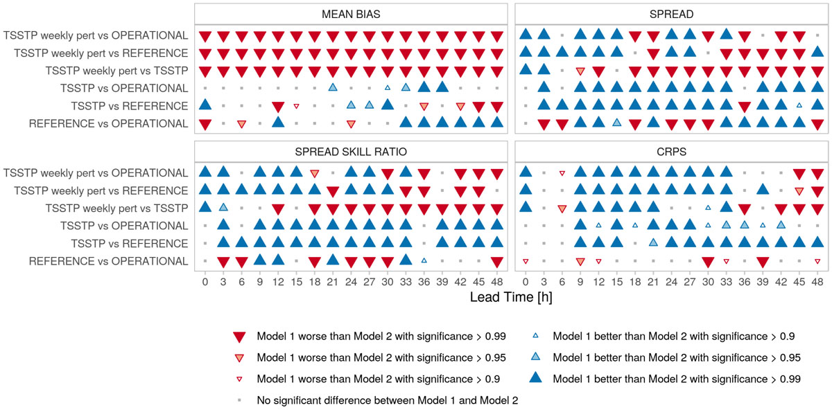
Figure 10
Comparison of the experiments regarding 2 m temperature.
REFERENCE shows mainly a larger spread compared to OPERATIONAL. TSSTP has higher spread compared both to REFERENCE and OPERATIONAL, while showing a lower spread when compared to TSSTP_weekly_pert. The comparison of TSSTP_weekly_pert to OPERATIONAL and REFERENCE shows mainly an increase in spread during the first 24 hours and mainly degradation thereafter.
The differences of the spread skill ratio reflect the differences in spread when comparing TSSTP, OPERATIONAL and REFERENCE due to a similar mean bias in all those three experiments. This is as well the case for the differences of the spread skill ratio of TSSTP_weekly_pert compared to the other three experiments. Even though TSSTP_weekly_pert shows a worse mean bias in all comparisons.
CRPS shows almost no significant differences between REFERENCE and OPERATIONAL. TSSTP seems to improve CRPS when compared to REFERENCE and OPERATIONAL. TSSTP_weekly_pert generally improves CRPS when compared to the other three experiments with some degradation during the last 6 to 15 hours.
The comparison of the experiments regarding 2 m specific humidity show similarity to the differences of 2 m temperature, and are displayed in Figure 11. Again, TSSTP_weekly_pert shows mainly a worse mean bias compared to all other experiments. REFERENCE seems to improve mean bias compared to OPERATIONAL from forecast hour 33 on, but shows a worse mean bias when compared to TSSTP for the same period.
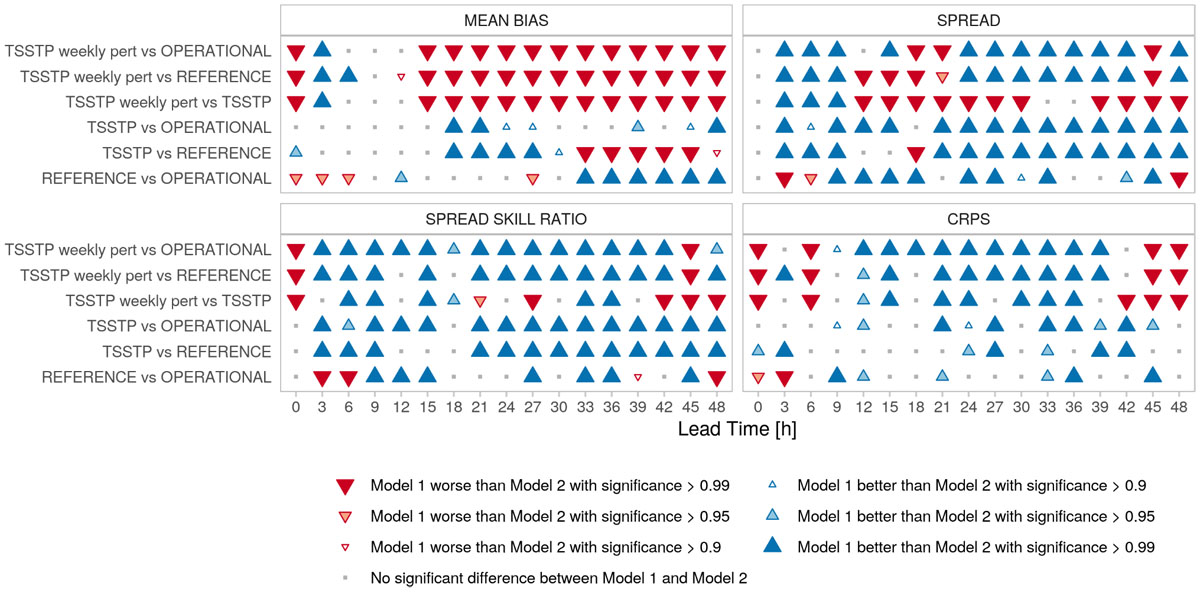
Figure 11
Comparison of the experiments regarding 2 m specific humidity.
TSSTP shows a larger spread and spread skill ratio when compared to both OPERATIONAL and REFERENCE. While REFERENCE shows improvement over OPERATIONAL for both those metrics. TSSPT_weekly shows a mainly larger spread when compared to REFERENCE and OPERATIONAL, but a smaller spread when compared to TSSTP. This is, however, not reflected in the spread skill ratio, where TSSTP_weekly_pert shows improvement over all other three experiments suggesting a lower RMSE.
In the case of CRPS, both TSSTP, REFERENCE and OPERATIONAL show less significant differences, and mainly improvement of TSSTP over both REFERENCE and OPERATIONAL. TSSTP_weekly_pert shows improvement over all three experiments in the period between 12 and 39 hours, and predominantly degradation before and after that period.
The results of comparing the experiments regarding 10 m wind speed can be seen in Figure 12. The differences in mean bias show some similarity to those of 2 m temperature and specific humidity. TSSTP_weekly_pert shows a worse mean bias compared to the other three experiments, while TSSTP shows no differences compared to OPERATIONAL, but degradation when compared to REFERENCE. REFERENCE however shows some improvement compared to OPERATIONAL.
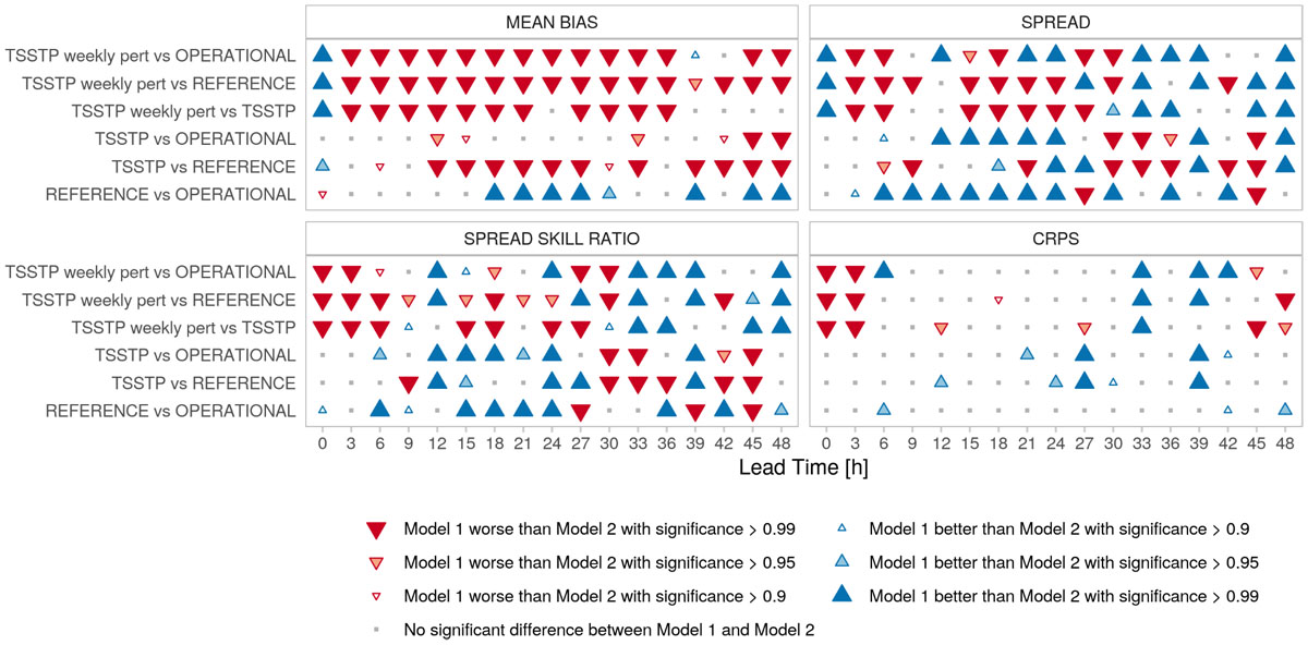
Figure 12
Comparison of the experiments regarding 10 m wind speed.
Both spread and spread skill ratio show a variation of improvement and degradation, depending on the forecast hour for most of the comparisons. TSSTP_weekly_pert predominantly seems to perform worse compared to the other three experiments. TSSTP shows little differences during the first 12 hours when compared with REFERENCE and OPERATIONAL. There is some indication that TSSTP shows larger spread and better spread skill ratio during the first half of the forecast compared with OPERATIONAL. REFERENCE in general seems to increase spread and thus improve spread skill ratio when compared to OPERATIONAL.
CRPS shows almost no significant differences for any of the comparisons, apart from TSSTP_weekly_pert showing consistently worse CRPS during the first 6 hours of the forecasts, and both TSSTP and TSSTP_weekly_pert showing some isolated cases of improvement over the other experiments during the last half of the forecasts.
3.3 Comparison of perturbations methods based on ASCAT wind observations
The comparison of the experiments based on ASCAT wind observations is displayed in Figure 13. REFERENCE and TSSTP generally increased the mean bias compared to OPERATIONAL. The comparison of TSSTP to REFERENCE indicated tendencies of a worse mean bias during the first half of the forecast periods and improvement thereafter. TSSTP_weekly_pert predominantly improved mean bias compared with the other experiments.
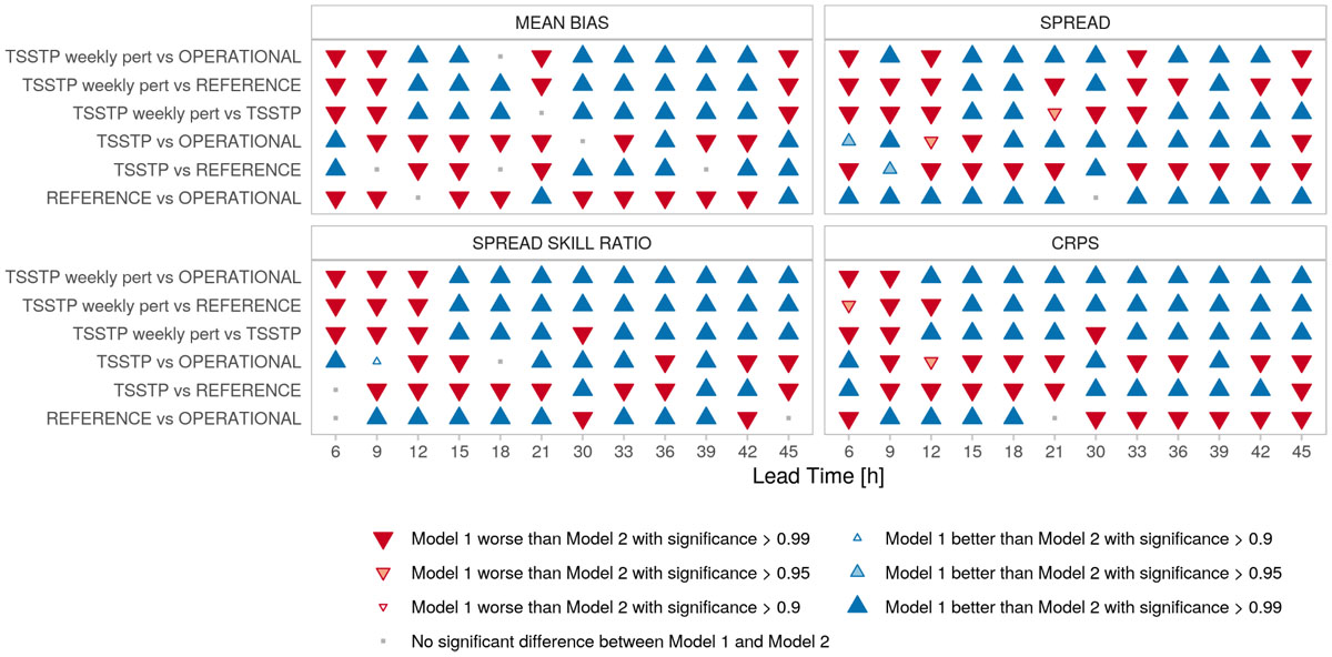
Figure 13
Comparison of the experiments regarding 10 m wind speed based on verification with ASCAT wind data.
Both REFERENCE, TSSTP and TSSTP_weekly_pert improved spread when compared to OPERATIONAL. REFERENCE showed increased spread compared to TSSTP for almost the entire forecast period, and increased spread for the majority of the period when compared to TSSTP_weekly_pert. The comparison of TSSTP_weekly_pert and TSSTP regarding spread shows mainly decreased spread during the first half of the forecast period and mainly increased spread thereafter.
The results for spread skill ratio indicate improvement for both TSSTP_weekly_pert, TSSTP and REFERENCE over OPERATIONAL. TSSTP_weekly_pert shows clear improvement for the whole period apart from the first 9 forecast hours over all other experiments. The comparison of TSSTP and REFERENCE shows a better performance and spread skill ratio for REFERENCE.
CRPS mirrors the differences of spread skill ratio in the case of TSSTP_weekly_pert. TSSTP shows a worse CRPS when compared to OPERATIONAL, and a worse CRPS during the first half of the forecast period followed by improvement when compared to REFERENCE. REFERENCE shows improvement of CRPS during the first half of the forecast period and degradation thereafter when compared to OPERATIONAL.
3.4 Comparison to operational analyses
The verification against operational analyses is split into scores for all grid points, for grid points over land, for grid points over open sea (sea ice concentration < 0.5 in the analysis) and for grid points over both sea and sea ice. As for the verification against SYNOP stations and ASCAT wind speeds, the scores were computed over all of the weather events in this study combined. Only the ensemble spread and RMSE are shown as they succinctly summarise the performance of the ensemble and of the differences between experiments discussed in this section are statistically significant by the bootstrap method.
Figure 14 shows the spread and RMSE for mean sea level pressure for all experiments, with the spread and RMSE for 10 m wind speed displayed in Figure 15. For both of these parameters, all experiments show only small differences in spread and RMSE both over land and sea. With regard to mean sea level pressure, all experiments have a spread that exceeds the RMSE, which is a known feature of the Harmonie EPS ensemble and SST perturbations have little impact overall on improving that.
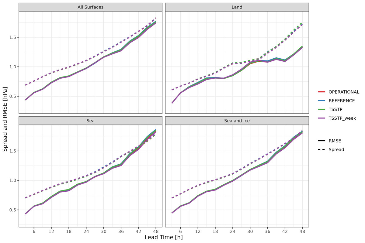
Figure 14
Spread and RMSE for mean sea level pressure.
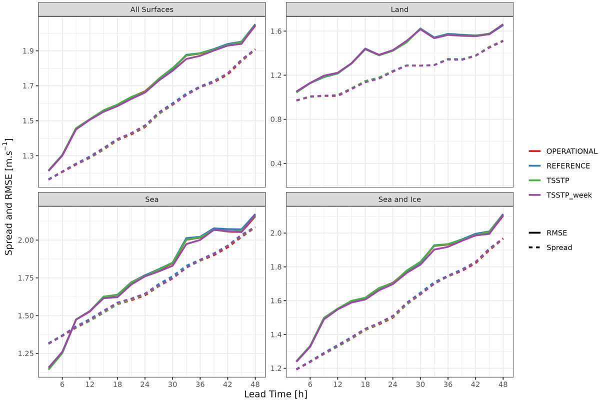
Figure 15
Spread and RMSE for 10 m wind speed.
Spread and RMSE for 2 m temperature are shown in Figure 16. Again, all experiments show rather similar RMSE and spread over land. Over the sea, however, the spread is biggest for TSSTP_weekly_pert, followed by TSSTP, REFERENCE and OPERATIONAL in that order. With the inclusion of grid points over sea ice TSST_weekly_pert shows a smaller RMSE on the first day of the forecast.
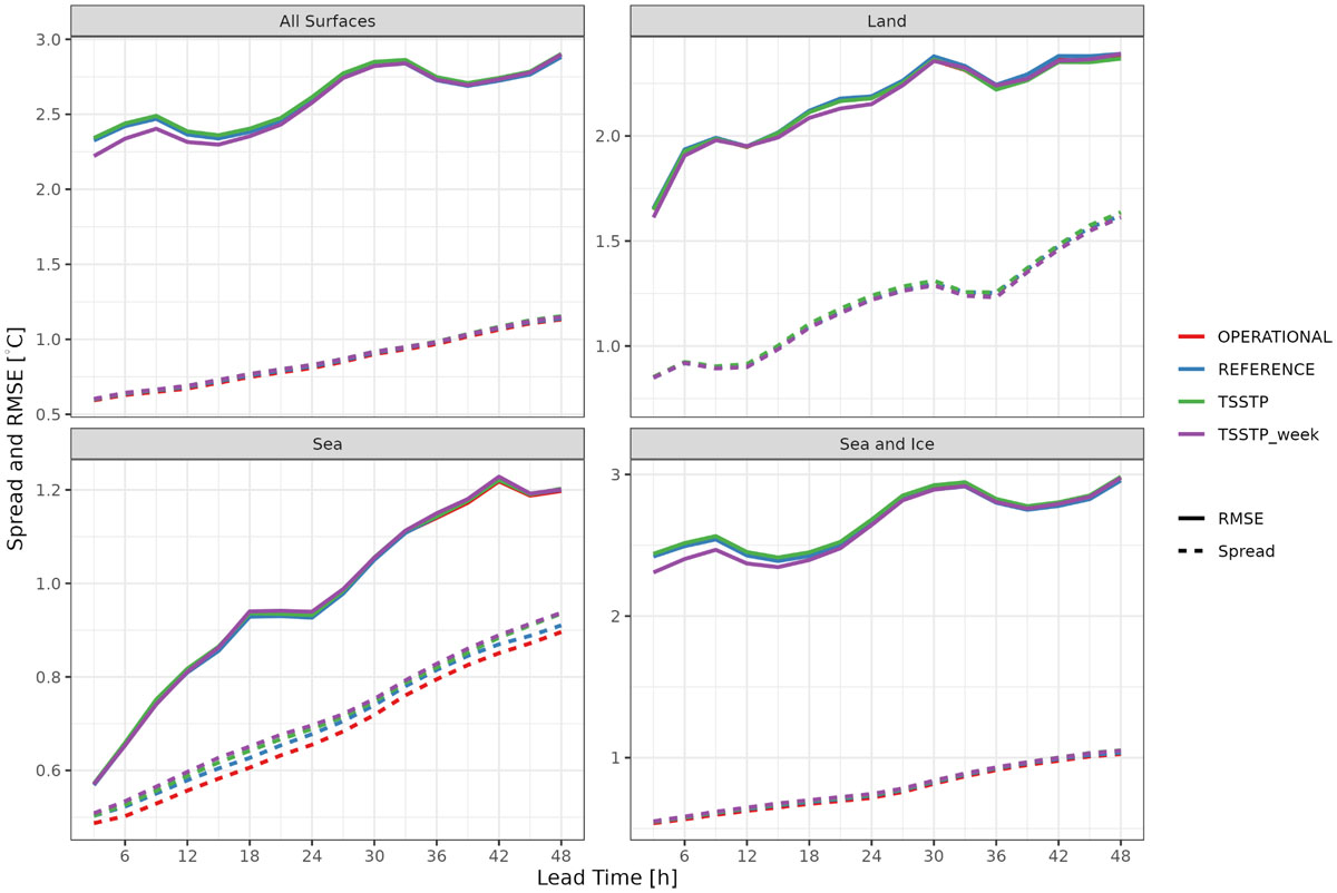
Figure 16
Spread and RMSE for 2 m temperature.
The differences for 2 m specific humidity (Figure 17) show, similar to 2 m temperature, similar RMSE and spread for all experiments over land, and differences in spread over sea as described for 2 m temperature. Though the differences seem to be overall smaller for 2 m specific humidity.
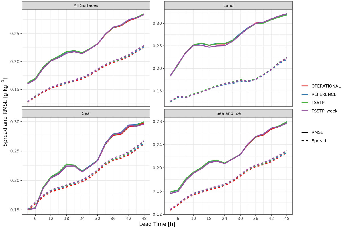
Figure 17
Spread and RMSE for 2 m specific humidity.
4. Discussion
In this research we aim to determine to what extent the location and magnitude of SST perturbations in a limited area EPS over the European Arctic impacts forecast performance for high impact weather. This question was addressed by running experiments with SST perturbations located randomly (OPERATIONAL and REFERENCE), and with SST perturbations targeted towards locations where the SST uncertainty was thought to be largest (TSSTP and TSSTP_weekly_pert). For the randomly located SST perturbations, the magnitudes of the perturbations were different in the two experiments. For the targeted perturbations, the experiments used different time periods for the estimation of SST uncertainty. Ensemble verification scores for the different perturbation setups were compared for near surface weather parameters observed at SYNOP stations over land, wind speed derived from ASCAT scatterometer observations over the ocean, and for parameters derived from operational analyses.
A bootstrap approach with 1000 replicates was performed to test the similarity of the verification results. The Kolmogorov-Smirnov test was chosen to find significant differences between the bootstrap samples of the experiments in this study. A property of the test is that it is sensitive to all types of differences between the distributions being compared, i.e. different medians, different variances, or different distributions, and as a result tends to have a smaller power compared to other significance tests. However, it has been shown that the power of the test can become very large when using large sampling sizes (Larson, 2018), leading to false rejections of the null hypothesis that both experiment scores stem from similar underlying distributions.
Since the only difference between the experiments is the structure and magnitude of the SST perturbations, it would be reasonable to expect an impact on the temperature over the sea. Verification against analyses from the operational AROME-ARCTIC model was done to assess the impact of the different SST perturbation strategies over the sea. Operational analyses were chosen as a reference against which to verify the experiments due to the lack of direct observations over the sea. Whilst an analysis cannot be considered to be as accurate as direct observations, it can provide a reasonable estimate against which to compare different modelling setups in the absence of in situ observations.
An increase in the spread for 2 m temperature over sea grid points (Figure 16) is seen as the magnitude of the perturbations increases from the OPERATIONAL to the REFERENCE experiments. As the locations of the perturbations become more structured in the TSSTP experiment a further increase in ensemble spread for 2 m temperature is observed, and finally as the locations of the SST perturbations become more targeted towards to the actual uncertainty in the SST in the TSSTP_weekly_pert experiment another increase in the 2 m temperature spread is seen. These increases in spread do not lead to any degradation of the RMSE for 2 m temperature and thus an improved spread-skill relationship is achieved over the sea. This means that both TSSTP and to a larger extent TSSTP_weekly_pert are generating SST perturbations in areas where the atmosphere is more sensitive to changes in the SST. An added advantage is that TSSTP_weekly_pert ensures that no perturbations occur in grid squares with sea ice concentration greater than zero, meaning that the RMSE over sea grid squares including sea ice is greatly reduced. Changes in sea surface temperature are also likely to impact evaporation and a similar, albeit smaller, increase in spread is seen for 2 m specific humidity as the perturbations increase in magnitude and become more structured towards specific locations (Figure 17).
The increases in ensemble spread for 2 m temperature and 2 m specific humidity suggest that there may be an impact on the sensible and latent heat fluxes which could influence the development of weather systems and have a downstream effect over the land. With this in mind, the impact of the different SST perturbation strategies was investigated against satellite derived observations of wind speed over the sea using scatterometer derived wind speeds and over land using observations from SYNOP stations. On the whole, small, but statistically significant differences for verification scores were found between the different SST perturbation methods suggesting that the chosen case studies were sensitive to changes in SST.
The verification against scatterometer winds (Figure 13) suggests that proper targeting of the SST perturbations has a positive impact on the ensemble forecast of 10 m wind speeds over the sea, with TSSTP_weekly_pert verifying better than the other perturbations for most lead times except for the first 9 – 12 hours of the forecast. In general increasing the magnitude of the perturbations improves the performance of the ensemble, with REFERENCE outperforming OPERATIONAL at the expense of a worsened bias, but targeting those perturbations towards areas of general SST uncertainty derived from annual estimates appears to have a detrimental effect (TSSTP vs REFERENCE). This means the way that the latent and sensible heat fluxes interact with the wind speed over the sea for the weather systems included in this study is sensitive to the locations of the SST perturbations.
The four weather events included in this study developed and were mostly active over the sea. This means that the impacts of SST perturbations on verification scores for SYNOP stations over land were either related to downstream effects from the large scale weather system, or more localised atmospheric responses.
The results showed a variation of improvements in the case of mean sea level pressure. While it appears that TSSTP and REFERENCE increased the mean bias of the model, they also had a positive impact by increasing the spread. However, the increased spread was not able to outweigh the degradation due to the increased mean bias. This becomes also apparent in a general poorer CRPS for both experiments. TSSTP_weekly_pert showed slightly different results where mean bias showed some improvement while spread was decreased, leading generally to an improvement of the spread skill score. Further, it showed a periodic behaviour of improvement and degradation for CRPS, where improvement seems to be connected to daytime and degradation to night time. Although statistically significant, the magnitudes of these changes are very small as suggested by the RMSE for mean sea level pressure over land (Figure 14).
For 2 m temperature and 2 m specific humidity, the experiments with increased perturbation amplitudes (REFERENCE, TSSTP, TSSTP_weekly_pert) seemed to increase the spread, which led to an improved ensemble performance as indicated by the spread skill ratio and the CRPS for TSSTP. In the case of REFERENCE the increased spread did not necessarily lead to an improved spread skill ratio or CRPS. TSSTP_weekly_pert also showed a statistically significant increase of mean bias at all lead times for 2 m temperature and most lead times for 2 m specific humidity. This suggests that the targeted SST perturbations may be unbalanced. Over infinite ensemble members a well balanced perturbation strategy should tend towards a value of zero at each grid point. The mean perturbations for each of the SST perturbation methods (Figure 18) suggest that there is a tendency towards warmer perturbations around the north Norwegian coast, and it may be this that is impacting the bias. However, given that this is a limited number of cases and only ten ensemble members it may not be the case if more time periods were included in the analysis. Additionally, there may be a disconnect between the SST perturbations and the soil temperature perturbations over the land that results in a bias. The SST perturbations in REFERENCE and OPERATIONAL use the same perturbation pattern as the soil temperature perturbations over land following Bouttier et al (2016) whereas there is no relationship between the SST perturbations and the soil temperature perturbations over land for TSSTP and TSSTP_weeklyy_pert. However, if this disconnect were the source of the poorer mean bias it would also be reflected in the mean bias for TSSTP.
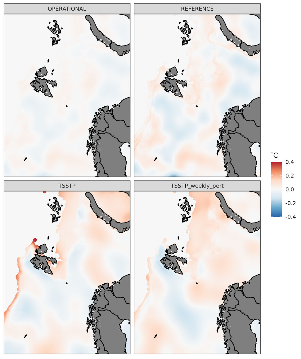
Figure 18
Mean SST perturbations for each of the perturbation methods averaged over all forecasts.
The results for 10 m wind speed based on SYNOP observations indicated an increased mean bias for TSSTP and TSSTP_weekly_pert but no consistent improvement of spread, leading to very mixed results for the spread skill ratio and almost no significant differences for the CRPS. Only the REFERENCE experiment showed improvement in mean bias and spread, but lacked any improvements in CRPS. However, the comparison based on ASCAT wind observations indicated improvement in mean bias and some improved spread for TSSTP_weekly_pert, leading to an overall better EPS performance as indicated by spread skill ratio and CRPS. The same observation could not be made for TSSTP and REFERENCE. Both show an increased spread as well, but due to increases in mean bias, the improvement in spread did not lead to improvement of the spread skill ratio or CRPS in the case of TSSTP, or to consistent improvements of CRPS in the case of REFERENCE.
The improvement of REFERENCE, TSSTP and especially TSSTP_weekly_pert over OPERATIONAL suggest that for the Arctic Ocean, larger SST perturbations are needed for forecasts of 2 m temperature, 2 m specific humidity and wind speed than for other domains for which the EPS had been optimised (Frogner et al., 2019). Additionally, it seems that the increased amplitude of the perturbations rather than the exact placement of uncertainty is of more importance for coastal areas, since all three experiments showed improvement for the mainly land based SYNOP observations and TSSTP_weekly_pert did not perform better compared to TSSTP or REFERENCE.
5. Conclusions
Two general methods to perturb SST in an ensemble prediction system (Harmonie EPS) were compared for a domain over the Nordic Arctic using four weather events that were thought to be influenced by SST. One method distributes the perturbations randomly and the other attempts to target the perturbations towards areas where the SST is thought to be most uncertain derived from comparisons between a high resolution SST product that is not available in real time and the SST analysis used in the model. Four experiments were done: OPERATIONAL, which scaled the magnitude of SST perturbations following operational implementations of Harmonie EPS; REFERENCE, which used the same perturbation pattern as OPERATIONAL, but increased the magnitude of the perturbations; TSSTP, which used a perturbation pattern derived from annual uncertainty estimates of SST and is therefore representative of the general uncertainty in SST; and TSSTP_weekly_pert, which used a perturbation pattern derived from uncertainty estimates of SST for the week preceding the forecasts. The magnitude of the perturbations in REFERENCE were scaled such that the L1 norm of the perturbations was approximately equal to that for TSSTP and TSSTP_weekly_pert. In this way differences between the results of the REFERENCE, TSSTP and TSSTP_weekly_pert experiments were only due to the locations of the SST perturbations.
The importance of specific SST uncertainty estimates and targeting those uncertainties when generating perturbations becomes apparent in the verification of wind speed against ASCAT scatterometer observations over the sea and the verification against operational analyses over parts of the domain. Over the sea, TSSTP_weekly_pert was able to outperform all three models by improving the spread of the ensemble while not impacting the RMSE and improving the bias of the ensemble mean. Over land, however, targeting SST perturbations has a more mixed impact. The spread is generally increased without impacting the RMSE resulting in an improved spread-skill relationship, but TSSTP_weekly_pert introduces a bias in 2 m temperature, 2 m specific humidity and 10 m wind speed, which may be due to a tendency towards warmer SST perturbations upstream of the coast. Further investigation over more cases would be required to understand whether this tendency is systematic.
Sea surface temperature plays an important role in processes involving convection in the Arctic, as is the case for the development of polar lows or showers during a cold air outbreak. The comparison of perturbations for each experiment for the four case study periods shows that both OPERATIONAL and REFERENCE had rather homogeneous perturbation fields only different in the perturbation amplitude, while TSSTP and TSSTP_weekly_pert showed isolated areas of increased perturbations. The comparison of these perturbations with the synoptic situations showed that the locations of the largest perturbations were collocated with the areas that were important for the weather development, that is the area where the polar low formed for the PL case; the area south of the ice edge where cold polar air masses get into contact with the ocean surface in the CAO I case, less so in the CAO II case; and the area west of the low pressure system where a lot of shower activity developed for the STR case. This had probably a positive effect on the spread. The areas of largest SST uncertainty do not necessarily always collocate with the most active weather development, although it was partially the case in this study. However, targeting the areas with the largest SST uncertainty when generating perturbations might have dampened the bias introduced through perturbations where the uncertainty is small.
In summary one can conclude that AROME-Arctic displayed some improvement in the case studies presented through the introduction of targeted sea surface perturbations, The choice of uncertainty estimates for the generation of SST perturbations has an impact on the ensemble system, and situation specific uncertainty estimates should be used where possible. This study investigated mainly situations that are sensitive to sea surface temperature. The effects of targeted sea surface temperature perturbations on the model for longer periods including all possible weather scenarios should be the topic of future studies.
Acknowledgements
This work was funded by the Norwegian Research Council Project (280573) ALERTNESS – ‘Advanced models and weather prediction in the Arctic: enhanced capacity from observations and polar process representations’.
ASCAT data from EUMETSAT Ocean and Sea Ice Satellite Application Facility, Metop-B/C ASCAT coastal Winds 2012-onwards, OSI-104-b/OSI-104-c, extracted on 2021-11-19 from the EUMETSAT data centre https://archive.eumetsat.int).
Competing Interests
The authors have no competing interests to declare.