
1 Introduction
The study of how changing climate changes weather patterns, especially extreme weather, requires some knowledge of historical weather patterns. Historical reanalyses like the Twentieth Century Reanalysis (20CR Compo et al., 2011; Giese et al., 2016; Slivinski et al., 2019) and the European Centre for Medium-Range Weather Forecasts (ECMWF) reanalyses ERA-20C (Poli et al., 2016) and CERA-20C (Laloyaux et al., 2018) attempt to reconstruct global weather patterns as far back as the nineteenth century using data assimilation (DA) – a class of methods for combining observational data with a forecast model to estimate the state and parameters of a dynamical system.
The further back in time one goes, the fewer are the observations available for use in a reanalysis. One class of weather observations that extends deeply into the historical record comes from the written reports of mariners. Records from voyages of the English East India Company, for example, stretch back to the seventeenth century (Brohan et al., 2012). Many of these records have been digitized and are available through the International Comprehensive Ocean-Atmosphere Data Set (ICOADS Freeman et al., 2017). Wind speed and direction are common observations, but early wind speed measurements were reported using qualitative language. The introduction of the Beaufort scale for wind speed in the early nineteenth century enables qualitative descriptions of wind speed to be converted to a quantitative scale, but early wind speed records have significantly greater uncertainty than wind direction measurements, and are not considered instrumental (Prieto et al., 2005; de Paula Gomez-Delgado et al., 2019). Wind direction measurements were recorded with high precision using accurate magnetic compasses with as many as 64 points. Unfortunately, wind direction is a strongly nonlinear function of the wind field, which makes it difficult to assimilate using standard ensemble Kalman filter (EnKF) data assimilation methods that work best for linear observations with Gaussian errors (Evensen, 2009). The goals of this investigation are to develop ensemble methods that can assimilate wind direction measurements, and to demonstrate, at least in an idealized model, the value in assimilating such measurements. These goals are in service of the larger goal of ultimately improving historical reanalyses and perhaps motivating the digitization of more historical observations of wind direction.
The plan of the paper is as follows. Two ensemble-based approaches to assimilating wind direction are described in section 2. The idealized dynamical model used in the tests is described in section 3. The data assimilation experimental configuration is presented in section 4, and the results of those experiments are presented and discussed in 5. Conclusions are offered in section 6. Figure data and simulation code are available (Grooms, 2023).
2 Wind Direction Ensemble Data Assimilation
We begin by setting notation. The state of the dynamical system is denoted x, with a subscript j to denote the value of x at time tj. Observational information at time tj is denoted yj. Our uncertainty about the state of the system before taking observational information into account is described by a Bayesian prior distribution; the probability density function (pdf) associated with this distribution is denoted [x] and a random variable with pdf [x] is denoted X. The observation y is a draw from an observational distribution with pdf [y|x]. Viewed as a function of y this is the pdf of the observational distribution; viewed as a function of x it is proportional to the Bayesian likelihood. The goal of ensemble data assimilation is to draw samples x(n), which together form an ensemble , from some distribution that approximates the Bayesian posterior [x|y].
Ensemble Kalman filters (EnKFs) approximate the joint distribution of X and Y as Gaussian, which implies that the Bayesian posterior (which is simply a conditional of the joint distribution) is also Gaussian with well-known formulas for the posterior mean and covariance. To wit, if the parameters of the joint distribution are
then the posterior mean and covariance are
The Kalman filter (KF) formulas on which EnKFs are commonly based make a further assumption about the relationship between the state and observations, namely that
where ϵ is a centered Gaussian independent of X and with covariance R, and H is a matrix. This assumption, which is necessary for the KF but not for EnKFs, implies
which allows the recovery of more familiar KF update formulas.
In the context of wind direction observations, y is an angle and Y is a circular random variable. The assumption of joint Gaussianity at the heart of EnKFs is a severe limitation in this context, since circular random variables are simply not Gaussian. Indeed, when the measured wind direction is recorded on a 16, 32, or 64 point compass, Y is also a discrete random variable, which further underscores that it is not Gaussian.
In principle an EnKF assimilating wind direction can be implemented using a nonlinear observation model
where h is an arctangent that maps the wind vector to the wind direction. Though algorithmically straightforward, this approach implicitly treats Y as a Gaussian variable, rather than a circular one, by relying on the usual formulas for means and covariances of linear variables. The performance of this type of method is expected to be erratic at best. For example, consider an ensemble of two directions: ±7π/8 radians, i.e. west by northwest and west by southwest. A standard EnKF approach to nonlinear observation operators will treat the mean wind direction as eastward when it should be westward, and will consider the ensemble spread to be large when it is in fact small.
This section develops two ensemble data assimilation approaches for assimilating wind direction measurements. The first, presented in section 2.1, is based on an observation model for wind direction that takes the form (4), which allows the use of standard EnKF or variational methods. The second, presented in section 2.2, uses a two-step approach to ensemble data assimilation based on the seminal approach of Anderson (2003), as expanded recently by Grooms (2022). The two approaches are fundamentally distinguished by the way in which they deal with the wind direction observations. In the first approach, the wind direction observations are assimilated by constraining to zero the component of wind perpendicular to the observed wind direction. In the second approach, the wind direction observations are assimilated by rotating the wind direction towards the observed direction. The mathematical structure of the first approach makes it amenable to implementation via standard EnKF methods, while the structure of the second approach requires a more sophisticated implementation via a two-step ensemble filter.
2.1 EnKF for Wind Direction
The goal of this section is to develop an observation model that approximates the true likelihood associated with a wind direction measurement, and that is amenable to incorporation into standard EnKF-type methods. Let u = (u, v)T be a two-component horizontal wind vector with eastward component u and northward component v. If θ ∈ [–π, π) is the direction of u measured in radians counterclockwise from east, then
If u points in the direction θ, then
although the converse is not true; (10) only guarantees that u has angle θ ± π.
Equation (10) is reminiscent of the linear observation model (4) commonly used in EnKFs, where
It is interesting to note that this version of the observation model flips the usual paradigm upside down. In the usual paradigm the observation matrix H is fixed and the value of the observation is y. In the version adopted here the value of y is always zero, while the observation matrix H depends on the observed angle θ.
What’s missing here is an additive observation error ϵ. The choice of error variance is somewhat ad hoc, since the observation model is only an approximation. The approach to specifying ϵ developed here is illustrated in Figure 1. The true angular likelihood is illustrated schematically in Figure 1 as follows. A solid line emanating from the origin indicates the observed wind direction; uncertainty in the true wind direction (as distinct from the observed wind direction which may contain slight errors) is illustrated by dashed lines emanating from the origin and flanking the solid line. The approximate likelihood associated with the linear observation model (11) says that the component of wind perpendicular to the observed direction is zero, with some uncertainty. This is illustrated in Figure 1 as follows. The central dotted line is parallel to the observed wind direction, while the flanking dash-dotted lines indicate uncertainty in the magnitude of the component of the wind vector perpendicular to the observed wind direction. The uncertainty in the two likelihoods intersects at a particular flow speed ∥u∥. In the figure this flow speed is the radius of the circle that passes through the points where the dashed lines (uncertainty in the true likelihood) intersect the dash-dotted lines (uncertainty in the linear model). Choosing an observation error variance in the linear model is thus equivalent to choosing a flow speed such that the uncertainty in the linear model and angular model match.
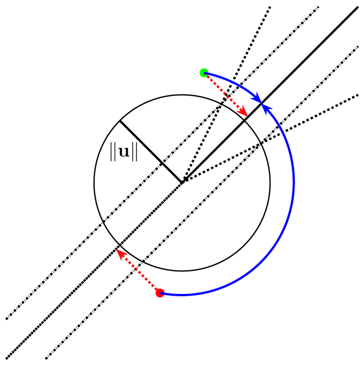
Figure 1
The solid line emanating from the center of the circle indicates the observed wind direction, while the dashed lines flanking the solid line indicate the uncertainty in the measurement of the wind direction. The dotted lines indicate the linear observation model: The central dotted line is parallel to the observed wind direction, and the flanking dotted lines represent the uncertainty in the magnitude of the wind perpendicular to the observed wind direction. The magnitude of the uncertainty in the linear model is chosen so that it matches the magnitude of the uncertainty in the wind direction at a particular wind speed; this wind speed where the uncertainties match is the radius ∥u∥ of the circle. The red lines indicate the way in which a wind vector (solid circles) is adjusted by the EnKF approach, while the blue lines indicate the way in which a wind vector is adjusted by the TSEF approach. The green solid circle is adjusted similarly by the EnKF and TSEF approaches, while the red solid circle is adjusted correctly by the TSEF and incorrectly by the EnKF.
Based on this geometrical motivation, the observational uncertainty in the linear model is set as follows. In the context of an EnKF, an ensemble of prior (forecast) wind vectors is available; in order to make the linear observation model accurate for a typical wind speed, the effective wind speed is set to
To get the observation error standard deviation in the linear observation model, we need the observational uncertainty in the angular measurement of wind direction. Naturally, historical observations of wind direction do not come with built-in quantification of their uncertainty, i.e. the true likelihood is unknown. The approach taken here, which can easily be modified, is to say that the standard error in measurements recorded on a compass with Nθ points is equal to half of a compass increment, i.e. π/Nθ. The arc length of a circular segment from the true wind direction to the true wind direction plus one standard error at a wind speed of ∥u∥ is ∥u∥ × π/Nθ. The observational error variance in the linear model is thus set to the square of this arc length
With this linear observation model, the wind direction observation can be assimilated by any one of the wide variety of EnKF methods available in the literature, or even using variational methods. The EnKF experiments reported here use the serial square root assimilation scheme of Whitaker and Hamill (2002). To distinguish this specific EnKF algorithm from other EnKFs, the serial square root assimilation will hereafter be denoted ESRF (Ensemble Square Root Filter). In a situation where wind speed measurements are available but with a much lower precision than wind direction, e.g. because the wind speed observation is simply the phrase ‘light wind’ (Brohan et al., 2012), the component of wind in the observed direction could be assimilated using an appropriately large error variance; this would be equivalent to observing both components of wind, but with a non-diagonal 2 × 2 observation error covariance matrix. Some historical observations of wind direction are unclear about whether the recorded direction is the direction from which the wind blows or to which the wind blows (Freeman et al., 2017); since the linear observation model is exactly the same for angles θ ± π, this method can still use wind direction observations that are subject to this ambiguity.
2.2 A Two-Step Ensemble Filter
Anderson (2003) developed a two-step approach to assimilating scalar observations that are nonlinearly related to the state by a relation similar to the linear observation model (4), namely
The first step of this two-step approach consists of a Bayesian estimation of h(X), while the second step consists of a simple linear regression from h(X) back to X. In the original implementation, the first step used the ensemble adjustment Kalman filter (EAKF Anderson, 2001); more recently, methods like the Rank Histogram Filter (RHF Anderson, 2010) and the GIGG-EnKF (Bishop, 2016) have been developed for the first step to relax the Gaussian approximation of the original EAKF. The second step typically uses simple linear regression, although generalized regression methods have been developed (e.g. Anderson, 2019). A key aspect of these methods is that they are algorithmically similar to EnKFs, and can be used efficiently with large-scale geophysical models (Anderson et al., 2009).
Grooms (2022) showed how two-step ensemble filters (TSEFs) are related to Bayesian estimation. A new random variable Z is introduced that has the property
In the context of the observation model (14), Anderson (2003) chose to use Z = h(X), but this is not the only possible choice of Z that satisfies the property (15). An illustrative but impractical alternative is to set Z = X; another choice is made below in the specific context of observations of wind direction. The introduction of this new variable allows the pdf of the Bayesian posterior to be written as
Two-step ensemble filters sample from this distribution by first sampling an ensemble from [z|y], and then sampling an ensemble where x(n) is a sample from [x|z(n)].
In the context of wind direction assimilation, let z = u and y = θ. It is convenient to change to polar coordinates for the wind vector, (u, v) ⟼ (ρ, ϕ) where the notation ϕ has been adopted to distinguish a general angle ϕ from the observed value θ. Note that in the context of the first step of the two-step filter, which is being described here, the choices z = u and z = ϕ work equally well; the choice z = u is made here because it leads to a better second step, which is described at the end of section 4. The posterior in polar coordinates is
While in general there is no reason to assume that ρ and ϕ are independent in the prior distribution [ρ, ϕ] = [ϕ][ρ], it is a highly convenient approximation, which is adopted here. Further assuming that the likelihood of observing the wind direction θ does not depend on the wind speed ρ, the posterior simplifies to
The assumption that ρ and ϕ are independent in the prior implies that the observation of wind direction has no impact on the distribution of wind speed. This assumption could potentially be relaxed by using the methods of Murphy et al. (2022), who, in a context different from data assimilation, model the conditional distribution of wind speed given wind direction [ρ|ϕ] as a Weibull distribution whose parameters depend on ϕ.
With these simplifying assumptions, the first step of the two-step process updates the direction of the wind vectors at the location of the observation while the second step uses regression to push the local changes in the wind vector back to all the other state variables. In this paper, the second step of the two-step process uses linear regression, as in the two-step EnKF of Anderson (2003). The first step is accomplished using a probability integral transform, which is the same idea that underlies the RHF and the Quantile-Conserving Ensemble Filter Framework (QCEFF; Anderson, 2022). If F– and F+ are the cumulative distribution functions (cdfs) of the prior and posterior, respectively, then the random variable is the probability integral transform of X– (which is distributed according to the prior), and X+ is distributed according to the posterior. To build a scalar filter for the first step of a two-step ensemble filter based on the probability integral transform, one uses the prior ensemble and the likelihood to approximate the cdfs, and then applies the resulting approximate transform to the prior ensemble.
In the context of wind direction, which is a circular random variable, the probability integral transform can still be used, though the definition of the cdf requires a small amount of care. For a random variable X taking values in , the cdf is defined to be
where ξ is a dummy integration variable and [X = ξ] is the pdf of X evaluated at ξ. For a circular random variable ϕ, one can define the cdf as
for any ϕ0. The choice of ϕ0 determines the domain of Fϕ, which is [ϕ0, ϕ0 + 2π].
To approximate the prior pdf [ϕ], we use kernel density estimation with a von Mises kernel (Mardia, 1975)
where I0 is the modified Bessel function of the first kind and order 0. The parameter κ controls the width of the kernel; for large κ and for ϕ ∈ (–π, π) the kernel approximates a normal distribution with mean zero and variance κ–1. The prior pdf is thus approximated from the prior ensemble as
where is the ensemble of prior wind directions. The kernel bandwidth parameter κ is set using a standard bandwidth selection scheme for Gaussian kernels (Silverman, 1998), adapted to the von Mises context:
where
Improved bandwidth selection schemes for von Mises kernel density estimation are discussed by Tenreiro (2022).
The domain of the prior cdf F– that is required for the probability integral transform is chosen to be [θ–π, θ+π] where θ is the observed wind direction. The prior cdf F– is approximated using trapezoid rule quadrature on an equispaced grid of 257 points in [θ–π, θ+π]. Linear interpolation is used to approximate F– between these 257 points. To obtain the posterior cdf F+ that is required for the probability integral transform, the posterior pdf is first evaluated as the product of the prior pdf and the likelihood on the same set of 257 points in [θ–π, θ+π]. Trapezoid rule quadrature is then used to obtain an approximation to F+ on the grid, and linear interpolation is used to fill in the intermediate values. The cdf is inverted by simply swapping the role of the ordinate and abscissa in the linear interpolation scheme used to evaluate F+. The form of the likelihood used in the experiments is discussed in section 4.
2.3 Example
This section presents a simple example to illustrate the differences in the first step of the EnKF and TSEF methods. In practice there would be many observations of wind direction at different locations, each of which would be serially assimilated into the state vector. The example presented here illustrates only the first step of the assimilation for a single observation of wind direction, and in this example the observed wind direction is very different from the wind directions in the forecast ensemble. An ensemble of N = 72 wind vectors are drawn from a random distribution – specifically, from a randomly-chosen spatial location in the initial distribution of the experiments described in section 4. This initial ensemble is shown as blue dots in the right panel of Figure 2. The estimate of the prior pdf produced by the von Mises kernel density estimation is shown as a blue line in the left panel of Figure 2. For ease of visual comparison with the posterior, the prior pdf has been scaled to have a maximum height of 1.
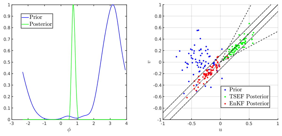
Figure 2
Left: The prior (blue) and posterior (green) pdfs of angle ϕ. Both are normalized to have unit maximum height so their shapes can be compared more easily. Right: A prior ensemble of wind vectors (blue), together with the posterior ensemble of wind vectors produced by the probability integral transform approach (green) and the EnKF approach (red). The solid black line is in the direction of the observed wind; the dotted black line is opposite to the direction of the observed wind; the dashed lines enclose the directions with nonzero likelihood; and the dash-dotted lines enclose the 95% confidence interval associated with the EnKF observation model.
The observed wind direction is set to θ = π/4, i.e. towards the northeast. This is shown in the right panel of Figure 2 by a solid black line emanating from the origin, while the dotted black line points in the opposite direction 5π/4. The posterior pdf, normalized to a maximum height of 1, is shown in green in the left panel of Figure 2; the likelihood used to form the posterior is given by Equation (31). The example uses a Nθ = 32 point compass so that the likelihood is nonzero only over an interval of directions of width 3π/16. The posterior is nearly equal to the likelihood in this example because the prior is so widely spread compared to the likelihood.
The probability integral transform rotates the prior wind ensemble members into posterior wind ensemble members, shown in green in the right panel of Figure 2, which is concentrated around the observed wind direction. The likelihood is identically zero for directions far from the observed value of π/4. The range of directions with nonzero likelihood is shown by a pair of dashed lines emanating from the origin in the right panel of Figure 2: The likelihood is zero outside these lines, and all of the posterior wind ensemble members lie between these lines.
The EnKF approach instead reduces the component of wind that is orthogonal to the observed wind direction; in this example the result is a posterior ensemble, shown in red in the right panel of Figure 2, whose members mostly point in the direction opposite to the observed direction. The EnKF uses an approximate observation model with an additive observation error set by Equation (13). The dash-dotted lines in the right panel of Figure 2 are located two standard deviations of the observation error above and below the observed direction, and most of the EnKF posterior ensemble members lie between these lines. This example illustrates that the EnKF approach does not work well for prior ensemble members that are pointing in the wrong direction.
To understand this result, Figure 1 illustrates how the ESRF and TSEF approaches update the wind direction vector in the first step of the two-step process. For a prior wind vector that is already close to the true observed wind direction (green dot) the TSEF rotates the wind vector without changing its amplitude (blue arc), while the ESRF projects the wind vector towards the right direction while minimally changing its amplitude (red arrow). The difference between the two methods is small when the prior wind vector is already close to the right direction. For a prior wind vector that is far from the observed direction (red dot), the TSEF again rotates the wind vector towards the observed direction without changing its amplitude (blue arc). The ESRF instead projects the wind vector in the wrong direction (red arrow).
3 Idealized model configuration
The wind direction data assimilation methods developed in the preceding section are applied here in the context of nondimensional two-dimensional incompressible vorticity dynamics on a β-plane. The vorticity ω evolves according to
The streamfunction ψ is proportional to a geostrophic pressure anomaly and will henceforth be referred to as pressure; it is related to vorticity by . Vorticity advection is represented via the Jacobian where . The coefficient β = 10 is the nondimensional meridional gradient of planetary vorticity. The domain is a periodic square with a nondimensional width of 2π. To convert the model state, i.e. vorticity, to wind direction at a given location requires a sequence of steps. First the Poisson equation is solved to find the streamfunction; then the components of velocity are obtained from the gradient of ψ via ; finally, the wind direction is obtained as the argument (sometimes called the phase or angle) of the complex number u+iv.
The forcing F is stochastic. It is Gaussian and white in time. Its spatial Fourier coefficients are nonzero only for wavenumbers with . On these wavenumbers the amplitude of forcing is constant; the value is chosen so that the net enstrophy injection rate is unity (nondimensional). Energy and enstrophy injected by the forcing are dissipated by a linear drag term with coefficient rd = 0.01 and viscosity with coefficient ν = 4 × 10⁻⁴.
The spatial discretization is a Fourier spectral method with 256 Fourier modes in each direction; the Jacobian is dealiased using the 3/2-rule, i.e. 384 Fourier modes in each direction are used in the computation of the Jacobian. The temporal discretization uses the fourth-order adaptive Runge-Kutta method ARK4(3)6L[2]SA of Kennedy and Carpenter (2003). All terms except the Jacobian are treated implicitly, while the stochastic forcing is added explicitly at the end of each Runge-Kutta step. The stepsize is adjusted using a PI.3.4 control (Soderlind, 2002) with a tolerance of 10–3. The code is publicly available (Grooms, 2023).
Figure 3(a) shows a snapshot of vorticity from the reference simulation. Eddies are mingled with zonal bands that correspond to zonal jets; the time- and zonal-mean velocity is shown in Figure 3(b). The energy spectrum is shown in Figure 3(c); a short inverse cascade produces a shallow spectrum between the range of forcing wavenumbers (shaded) and the peak of the energy spectrum at wavenumber 3, while the combination of linear drag and viscosity conspires to create a steep spectrum falling off from the forcing wavenumbers to the viscous dissipation range.
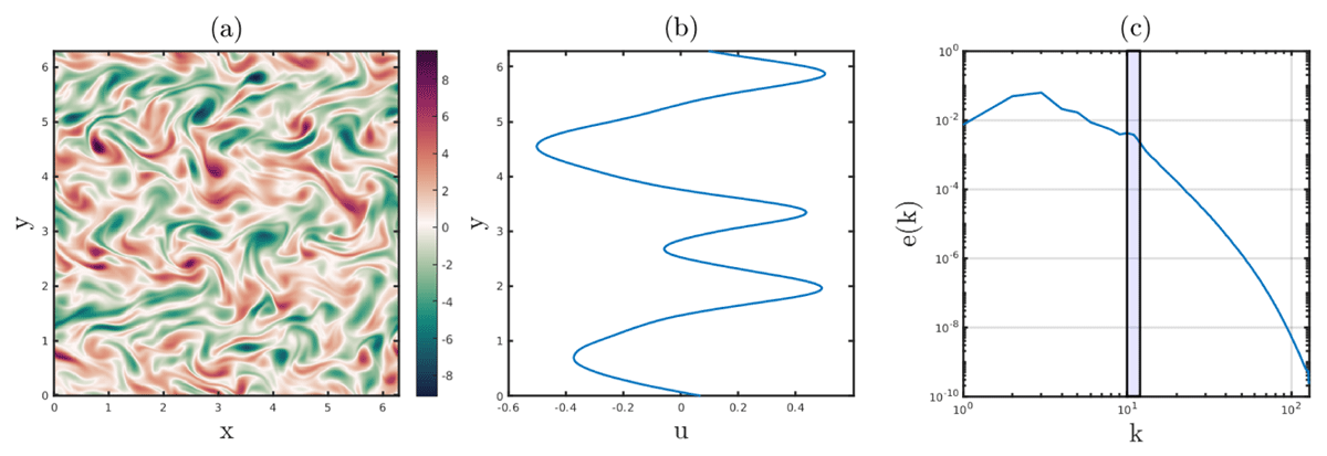
Figure 3
Properties of the reference experiment. (a) A snapshot of vorticity ω. (b) The time-mean and zonal-mean velocity profile. (c) The kinetic energy spectrum; the range of forcing wavenumbers is shaded. All variables are nondimensional.
4 Experimental Configuration
The data assimilation experiments reported here are designed to extrapolate, as far as possible for such an idealized model, to the setting of historical reanalysis. To that end, the observing system is spatially sparse: Observations are only available at 64 locations in the domain. In one set of experiments called ‘grid’ the observations are available on an equispaced 8 × 8 grid of points. The Nyquist wavenumber for this observing grid is wavenumber 4, which is between the forcing scale at wavenumbers 10–12 and the peak of the energy spectrum at wavenumber 3. In another set of experiments called ‘random’ the observations are taken at 64 randomly drawn locations throughout the domain, where the locations are drawn independently at every assimilation cycle.
The reference simulation was spun up from rest to a statistically steady state, at which point 1,024 reference states separated by 0.01 nondimensional time units were saved. Observations are assimilated every 0.01 nondimensional time units for the entire sequence of 1,024 reference states. These reference states constitute the ‘nature run’ used to make the synthetic observations and to evaluate the accuracy of the analyses. A fixed ensemble size of N = 72 was used, and the ensemble members were initialized as random draws from the time series of the reference state. The initial ensemble was the same for all experiments.
We perform a baseline set of experiments that assimilate only observations of pressure ψ. The observational error variance for ψ is 0.002, which is small compared to the climatological variance of 0.03. To assess the value of assimilating wind direction, we perform a set of experiments assimilating observations of wind direction in addition to observations of ψ, and another set of experiments assimilating only observations of wind direction. All experiments in the ‘grid’ configuration use exactly the same observations, and all experiments in the ‘random’ configuration share the same observation locations and values. For all configurations we assimilate wind direction using both the EnKF and TSEF schemes described in sections 2.1 and 2.2.
Localization is accomplished by multiplying the ensemble increments with a Gaussian localization function having a radius (i.e. standard deviation) of L. The radius L is chosen adaptively in a manner motivated by the approach taken in the third version of 20CR (Slivinski et al., 2019). Slivinski et al. (2019) argued that if an observation leads to a large increment of the state variable, then one might want to allow the increments to be spread over a wide region, whereas if an observation leads to a small increment of the state variable, then one might prefer to confine the increments to a small region. One motivation for such an approach is that a large increment confined to a small location is likely to produce large gradients and consequently dynamical instability. In the experiments developed here, the localization radius is set using
where
is the maximal increment to the pressure (subscripts – and + denoting prior and posterior, respectively). The smallest possible localization radius is four times smaller than the largest possible localization radius. Some initial tuning suggested that the localization radius should not be larger than 16 grid points, i.e. π/8 nondimensional units, so the maximal radius was set to
This maximal localization radius is half the shortest distance between the observation locations in the grid configuration. To standardize the different experiments, all experiments use the same formula for localization radius based only on observations of ψ. In experiments where observations of ψ are not assimilated, the increments to ψ that would result from observations of ψ are still computed solely for the purpose of setting the localization radius.
Also following 20CR, inflation used the ‘relaxation to prior spread’ (RTPS) inflation scheme of Whitaker and Hamill (2012). In this scheme the multiplicative inflation coefficient rinf is set to
where α is the RTPS parameter and σb and σa are the background (prior) and analysis (posterior) spreads, respectively. The relaxation coefficient α was manually tuned in each configuration to achieve optimal results. Inflation is applied to the analysis ensemble at each cycle.
Since historical observations do not come with a likelihood, we assume that the observation θ is obtained from
where denotes projection onto a compass with Nθ = 32 points and ϵ is the observation error, which is independent of u. This is clearly not in the form (14), but the TSEF framework of Grooms (2022) does not require (14), it only requires the likelihood [θ|ϕ]/[ϕ]. This is obtained, up to a normalization constant, by convolution of an indicator function I(ϕ) with the pdf of ϵ:
where πϵ denotes the pdf of ϵ and * indicates convolution. The indicator function I(ϕ) is zero for |ϕ| > π/Nθ and one for |ϕ| ≤ π/Nθ. The observation errors ϵ are here drawn from a symmetric triangular distribution peaked at zero and with a radius of π/16, i.e. the radius equals the precision of the 32-point compass. With this configuration of ϵ and a 32-point compass the likelihood is a quadratic B spline. The likelihood associated with this observation model could potentially be used to assimilate wind direction observations with local particle filters (Penny and Miyoshi (2016); Poterjoy (2016)).
The TSEF assimilates the observations serially, i.e. one at a time. For each observation there are two steps. The first step of the TSEF produces an analysis ensemble of wind vectors at the observation location. The second produces an analysis ensemble of vorticity fields . The update to the vorticity is accomplished using linear regression, following the approach of Anderson (2003), and explained in the Bayesian context by Grooms (2022). Let the vorticity values on the computational grid be unrolled into a vector x. A simple linear model is posited for the relationship between the vorticity vector x and the components u and v of the velocity vector u at the observation location
where a0,u,v are regression coefficients and η is the regression residual. The regression coefficients are obtained by plugging the prior ensemble into the simple linear model, and solving for the unknown regression coefficients using ordinary least squares. The estimates of the regression coefficients produced in this way are denoted , to distinguish them from the true regression coefficients. An ensemble of regression residuals can be defined using the estimated regression coefficients and the prior ensemble
where the subscript – serves to indicate that these values come from the prior ensemble. The analysis vorticity ensemble is then defined using the analysis velocity ensemble and the regression residuals as follows
This update can be written in incremental form as
where the increment is
Localization is accomplished by multiplying the increments by a localization function so that vorticity values far from the observation location are not updated.
Note that the choice z = u implies a regression problem in this second step where u is used as a predictor variable in the regression. The alternative choice z = ϕ, which works equally well in the first step, would require a second step where ϕ is used as a predictor variable in the regression. A first-order trignonometric polynomial model for the relationship between ϕ and x would take the form
This is similar but not equivalent to the model (32). The model (32) posits a linear relationship between the vorticity field x and the wind field u at a single point, whereas the model (37) posits a linear relationship between the vorticity field x and a unit vector (cos(ϕ), sin(ϕ)) in the same direction as the wind field u at a single point. The former model is more realistic (vorticity is related to wind speed and direction, not just wind direction), so the choice z = u is better than z = ϕ.
5 Results
The data assimilation results presented here are all given in terms of the root mean squared error (RMSE) in the vorticity posterior ensemble mean. Denoting the posterior ensemble in vorticity by , the posterior mean is
and the RMSE is
where the denotes an average in space or time and ω is the reference state from the nature run. Results showing the spatial pattern of RMSE use a time average, and results showing time series of RMSE use a spatial average. The analysis spread is defined to be
In all experiments the RMSE was only weakly sensitive to the RTPS parameter α, so it was tuned such that the spread matched the RMSE. Presenting results in terms of vorticity is convenient, but also somewhat more stringent of a test than considering alternatives like the pressure ψ or velocity u, since the latter are smoother fields than vorticity. Below we present results first for the grid observations, and then for the random observations.
5.1 Grid Observations
Results for the experiments with gridded observations are shown in Figure 4. The upper left panel shows the standard deviation of climatological variability in the reference simulation vorticity, with white crosses marking the locations at which observations are taken. The time- and space-mean standard deviation for the climatological variability is 2.17, but the variability is distributed non-uniformly through the domain in patterns associated with the zonal jets shown in Figure 3(b).
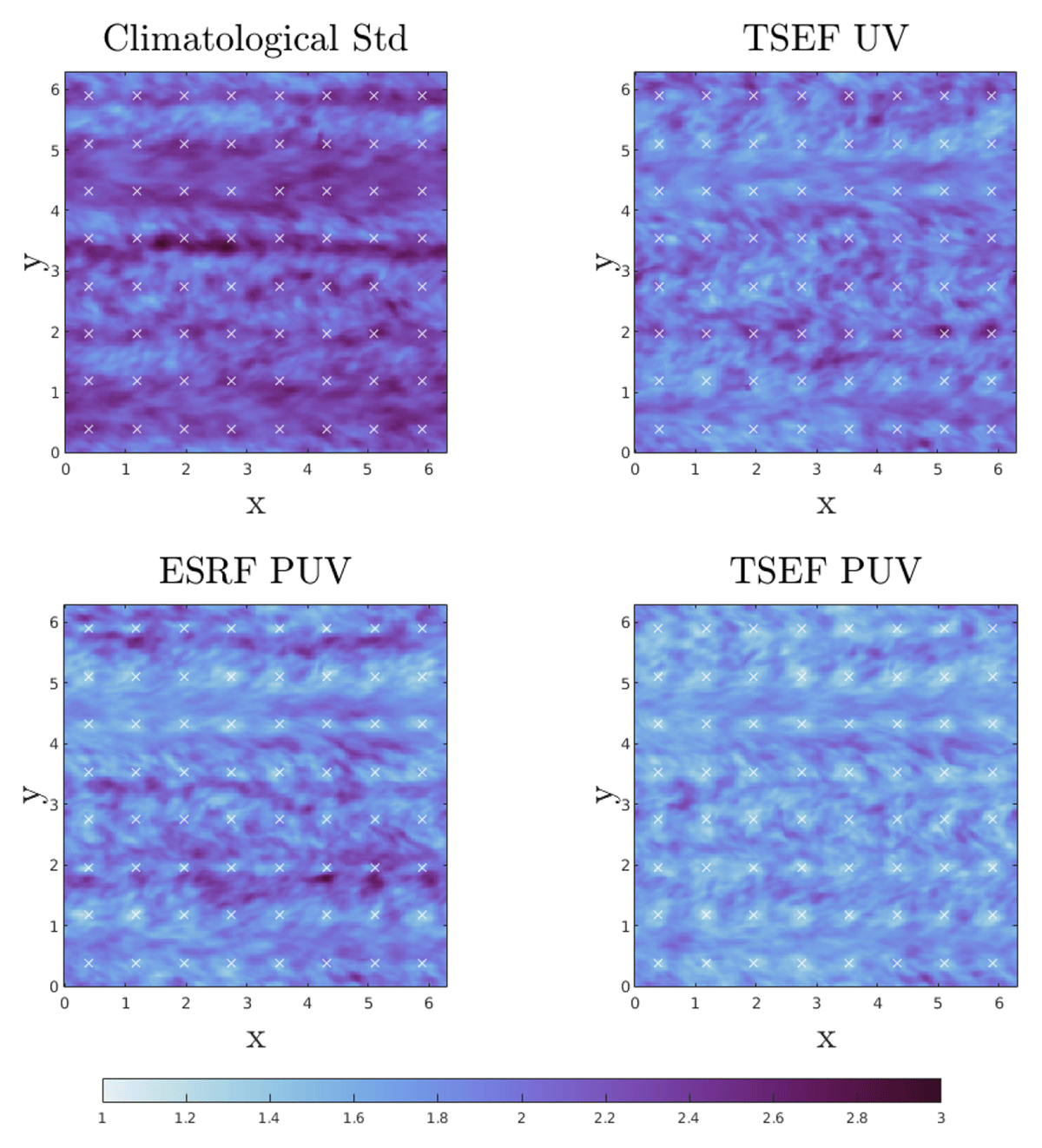
Figure 4
Upper left: Local standard deviation of climatological variability in the reference simulation vorticity. Upper Right: RMSE for the TSEF filter assimilating only wind direction. Lower Left: RMSE for the ESRF filter assimilating geostrophic streamfunction and wind direction. Lower Right: RMSE for the TSEF filter assimilating geostrophic streamfunction and wind direction. The white crosses in each figure are the locations of the observations.
The results for the ESRF and TSEF filters assimilating only pressure observations are essentially identical, and are not shown. Their RMSE is 1.85 at an RTPS value of α = 0.1. When assimilating only pressure observations, the TSEF is effectively a two-step EnKF, though not identical to the ESRF used in the other experiment, so it is not surprising that they yield indistinguishable results.
The lower panels of Figure 4 show the RMSE for the ESRF (left) and TSEF (right) filters assimilating both pressure and wind direction. Optimal results for both filters are obtained at an RTPS value of α = 0.3. The ESRF performs no better in this example than the ESRF that assimilates only pressure: they both have RMSE of 1.85. In contrast, the TSEF performs slightly better than the ESRF, with an RMSE of 1.7; this slight improvement is visible in the spatial pattern of RMSE shown in the lower right panel of Figure 4.
When assimilating only wind direction, the ESRF filter remains diverged (not shown). Across a range of RTPS parameters α from 0.1 to 0.9 the RMSE remains high, with an optimal RMSE of 2.34 at an RTPS value of 0.9. In contrast, the TSEF filter is able to perform nearly as well with only wind observations as it does with only pressure observations; the optimal RMSE of 1.9 is obtained at an RTPS value of α = 0.2. The spatial pattern of RMSE for the TSEF filter with only wind observations, shown in the upper right panel of Figure 4, is slightly better than the climatological pattern shown in the upper left panel.
In all cases the moderate performance of the filters, insofar as they improve only slightly over climatology, is because the observing system has been deliberately chosen to be sparse so as to be reminiscent of the sparsity of observations in the early centuries of a historical reanalysis.
5.2 Random observations
Figure 5 shows time series of the RMSE for both ESRF (left) and TSEF (right) filters with all three sets of observations (pressure only, pressure and wind direction, or only wind direction) with the random observation locations. As with the gridded observations, ESRF and TSEF perform indistinguishably when assimilating only pressure observations. Unlike the gridded observations, the ESRF and TSEF perform indistinguishably when assimilating observations of pressure and wind direction; for both filters, assimilating wind direction improves performance compared to just assimilating pressure. The big difference comes when assimilating only observations of wind direction. In this case, the ESRF diverges with RMSE above climatology, as it did with gridded observations, but the TSEF performs as well with only wind direction as it does with only pressure.
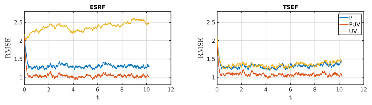
Figure 5
Time series of RMSE for the ESRF (left) and TSEF (right) filters with random observation locations. In the legend, P denotes experiments assimilating only observations of pressure, PUV denotes experiments assimilating observations of pressure and wind direction, and UV denotes experiments assimilating only observations of wind direction. The climatological standard deviation of vorticity is 2.17, for reference.
The results presented in Figure 5 use the following values of the RTPS parameter α: ESRF and TSEF assimilating only pressure α = 0.3; ESRF and TSEF assimilating pressure and wind direction α = 0.1; ESRF assimilating only wind direction α = 0.8; TSEF assimilating only wind direction α = 0.1.
5.3 Discussion
The main conclusion is that the TSEF performs as well using only wind direction observations as the ESRF does using only pressure. 20CR relies heavily on surface pressure observations since they are available deeply into the historical record; the results here suggest that similar performance might be possible using only wind direction observations. In contrast, the EnKF approach to wind direction provides no benefit when wind direction is the only observation.
To understand why the EnKF approach diverges when using only wind direction observations, assume that the prior uncertainty in the wind direction is high, as it would be in the early stages of a historical reanalysis. Figure 2 illustrates that the EnKF approach simply removes the component of wind orthogonal to the observed direction; for some ensemble members this is an improvement, while for others it is the opposite. With only this kind of observation, the EnKF approach is unable to reduce the uncertainty in wind direction, and remains diverged.
When other observation types are also available (e.g. pressure), these other observations can indirectly improve the accuracy of the prior wind direction. Then, with a reasonably-accurate prior, the EnKF approach can extract further value from the wind direction observations; this is most evident in the random-location configuration, where the EnKF performs better with wind direction and pressure than with pressure alone. Of course the TSEF approach is also able to perform better with wind direction and pressure than with wind direction alone.
The gridded observing system does not produce large differences in performance between the methods because none of the methods are able to perform very well. The limitation of that configuration is that the observations are sparse in the domain, and while the methods are able to accurately estimate the state close to the observation locations, the spatial correlations are not sufficient to spread the accuracy to the entire domain. The random observing system still has sparsely-spaced observations, but over time the observations cover the spatial domain uniformly, which leads to improved overall accuracy as well as a greater difference in the performance of the different methods.
As a result of this overall improved accuracy using randomly located observations, the prior ensemble in wind directions is more accurate than using gridded observations. This explains why the TSEF is slightly better than the ESRF with gridded observations while the methods perform similarly with randomly located observations: The prior wind ensemble is far more accurate with the randomly located observations, and the ESRF approach to assimilating wind direction works well with an accurate prior ensemble.
6 Conclusions
Two methods for assimilating wind direction observations have been developed for the purpose of enabling future historical reanalyses to make use of historical observations of wind direction. The first method uses a linear observation model and can be used with EnKF or variational approaches, while the second method is inherently nonlinear and non-Gaussian and requires an ensemble approach. The first step of the nonlinear TSEF approach uses a nonparametric ensemble approximation of a probability integral transform, and is thus an example of a Quantile Conserving Ensemble Filter (QCEF; Anderson, 2022). The nonlinear TSEF approach is amenable to implementation within the Data Assimilation Research Testbed software suite (DART; Anderson et al., 2009).
The two methods were tested in the context of an idealized two-dimensional fluid model. The main result is that the TSEF approach using only wind direction observations performs as well as an EnKF method using only pressure observations. Although the performance parity seen here depends on the details of the observing system, this is a clear demonstration that the new method can unlock latent value in historical measurements of wind direction. In contrast, the linear observation model provides no benefit at all when assimilating only wind direction observations.
The linear observation model is primarily valuable when used in concert with other observation types, e.g. pressure observations. If enough observational data is available to produce a reasonably-accurate forecast of wind direction, then the linear observation model for wind direction observations can be used to further improve the accuracy of the posterior estimate.
Acknowledgements
This research was funded by US National Science Foundation grant number DMS 2152814. The author is grateful to G. Compo and P. Brohan for introducing the author to the challenges of historical reanalyses, and to an anonymous reviewer for their constructive criticism. Figure data and code are available (Grooms, 2023).
Funding information
US National Science Foundation, Division of Mathematical Sciences, Grant Number: 2152814.
Competing Interests
The author has no competing interests to declare.