
1. Introduction
The “Navy Environmental Prediction sysTem Utilizing a Nonhydrostatic Engine,” referred to as NEPTUNE, is a new global weather prediction system being developed by the U.S. Navy, which is planned for operational implementation in the 2025 timeframe. NEPTUNE utilizes and extends the numerical methods prototyped in the “Nonhydrostatic Unified Model of the Atmosphere” (NUMA), a spectral element dynamical core (Kelly and Giraldo, 2012; Giraldo et al., 2013) based on memory-local, computationally dense numerics with near-ideal parallel scaling at high numerical order and large problem size (Michalakes et al., 2015).
In order to build an environmental prediction system with NEPTUNE, the dynamical core must be augmented with a suite of tools for forecast initialization, diagnostics, and observing network analysis. An essential part of this suite is a solver for the tangent-linearization of NEPTUNE, referred to as the tangent linear model (TLM), which can be used to approximate the evolution of small perturbations around a time- and space-varying background flow. Another part of this suite is a solver for the adjoint (ADJ) of the TLM, which is used to compute sensitivity functions with respect to the same time-dependent background. Both of these components are used in variational data assimilation algorithms (Courtier et al., 1993, 1994), but they are also useful in applications concerned with non-normal stability, quantification of observability and model sensistivity, and observation impact and observing system design (Errico, 1997; Langland and Baker, 2004; Luchini and Bottaro, 2014; Doyle et al., 2019).
In recent years there has been growing interest in the development of non-hydrostatic models to enable the same dynamical core to be used for regional mesoscale modeling, weather forecasting, and climate projection (Ullrich et al., 2017). Non-hydrostatic dynamical cores have been used within operational models for some time (Saito et al., 2006), and TLM and ADJ systems are available for some of them (Amerault et al., 2008); however, the development of variational initialization systems for their global application is an ongoing challenge due to the stringent performance requirements of global operational systems. For example, the TLM and ADJ of the finite-volume cubed sphere (FV3) dynamical core of the NASA Goddard Earth Observing System (GEOS) system is under active development (Holdaway et al., 2017). More recently, the TLM and ADJ of the unstructured-grid, finite-volume, Model for Prediction Across Scales (MPAS) was developed (Tian and Zou, 2020).
This paper reports on the development of the TLM and ADJ for the NEPTUNE dynamical core, which excludes the submodels for subgrid-scale turbulence, moist physics, chemistry, and radiative transfer used in the complete model. The key attribute of the NEPTUNE model is that it supports both continuous and discontinuous Galerkin expansions, with arbitrary order polynomial basis, on a cubed sphere spectral element grid. The NEPTUNE code has excellent scaling properties which are designed to enable its use on millions of compute nodes (Doyle et al., 2018). Similar performance is anticipated from the TLM and ADJ which utilize the same design principles as the NEPTUNE core.
2. Model Dynamics and Numerics
The dynamical core of NEPTUNE is a solver for the compressible Euler equations expressed in the form (Giraldo et al., 2010),
where the vector of prognostic varianbles, q = (ρ, uT, θ), consists of the density, ρ, the 3-component Cartesian velocity vector, u, and the potential temperature, θ. The Exner pressure is with gas constant R and reference pressure pA; the potential temperature θ is related to the temperature T by θ = T/π; and the equation of state relating pressure, density, and temperature is, p = ρRT. Finally, Ω is the planetary rotation vector, cp is the specific heat, and ɡ is the gravitational acceleration vector. This representation of the dynamics corresponds to equation set 2NC of Giraldo et al. (2010), with the modification that the pressure gradient is expressed in terms of the Exner pressure.
NEPTUNE utilizes a horizontally-explicit and vertically-implicit (HEVI) approach to efficiently integrate the discrete analogue of the above system (Giraldo et al., 2013; Gardner et al., 2018). The spatial discretization is obtained with Galerkin spectral elements (Giraldo et al., 2002) on a 3-dimensional cubed-sphere grid (Putman and Lin, 2007). The temporal and spatial discretizations used in the solver are described in more detail, below.
2.1 Temporal discretization
Following Gardner et al. (2018), equation (1) is time-stepped by additively splitting all but the time-derivative terms into two parts,
where fE and fI are the terms which are integrated explicitly and implicitly, respectively. Equation (2) is integrated from time tn–1 to time tn via a multi-stage additive Runge-Kutta (ARK) method of the form (Ascher et al., 1997),
where i = 1, …, s indexes the s-stage ARK method defined by coefficients, is the time step size, and and are intermediate times of the sub-stages. The zi vectors correspond to predicted values of q it the intermediate timesteps. Specifically, NEPTUNE implements the DIRK (3,4,3) algorithm (Ascher et al., 1997), referred to as the ARS343 integrator in the comparisons of Vogl et al. (2019).
The implicit components of the above splitting involve the solution of nonlinear equations to obtain zi,
where di is known from previous stages, and where the vertically-coupled dynamics responsible for sound and inertia-gravity waves are incorporated in the fI function. The HEVI approach combined with the ARS343 integrator solves the explicit horizontal dynamics with 4th-order accuracy, and the implicit vertical dynamics with 3rd-order accuracy (see Gardner et al. 2018 for details). The accurate representation of sound waves is not needed, but their inclusion keeps the dynamics strictly local in space and facilitates the scalable numerics.
A crucial point, relevant later in the development of the TLM and ADJ, is that the solver for equation (5) is based on Newton’s method and requires the product of the Jacobian of fI evaluated at with an arbitrary vector v,
The implicit part of the HEVI solver in NEPTUNE explicitly constructs the matrix A from the intermediate values of the fields, , using the Jacobian, J. In the TLM and ADJ solvers, the same strategy is employed for the linearized system; however, the implicit solver is strictly linear and evaluates the A matrix at qb, the time-dependent background trajectory around which the TLM linearization is defined.
2.2 Spatial discretization
To make the discussion of the TLM and ADJ specific, it is useful to write out the Galerkin spectral element method for a linear system, ignoring the details related to nonlinearity. Let q = q(x, t) be the vector characterizing the state of the system, and let x ∈ D be a position vector in domain D, and t ∈ [t0, t1] is the time. The evolution of the system is given by,
where L is the linear operator obtained from equation (1). Let be the space of polynomials up to degree p. If q ∈ , then a Galerkin method seeks to find q such that the error in (7) is orthogonal to . The solution vector q satisfies,
where,
is the inner-product over D, and ψ is any test function in .
The elementwise Galerkin expansion used in NEPTUNE is obtained by decomposing D into Ne elements, De, and performing a coordinate transform so that each element is defined over the unit cube ξ = (ζ, ξ, η) ∈ [–1,1]3 (Giraldo et al., 2002). Then (9) can be written as,
where the determinant of the metric tensor is,
Note that J and the transformation x(ξ) are implicitly functions of the element-index, e.
Let ϕi = ϕi(ξ) be the set of Lagrange polynomials in that interpolate the Gauss-Legendre-Lobatto (GLL) points ξi. Then the coefficient vector and q(ξ, t) are related by,
where qi,e(t) = q(x(ξi), t) for x ∈ De. With ψ = ϕj as a test function, substitute (12) into (8) and use (10) to get,
Although the inner product, equation (10), contains the sum over Ne elements, the Lagrange polynomials are non-zero only inside their element, and equation (13) is satisfied on each element independently. Using Gaussian quadrature to numerically evaluate the integrals in (13) yields,
where wl are the integration weights, |Jl| is the Jacobian transform matrix evaluated at the integration points, and the diagonal mass matrix is given by,
with the implicit dependence of J on e suppressed. Since ϕi is a Lagrange interpolating polynomial, the right-hand side of (14) is only non-zero for l = j, so it can be simplified to,
The GLL points are defined at element boundaries, which may be shared by several elements in the 3-dimensional grid. To assemble the global solution with unique values at all quadrature points, the solution procedure in NEPTUNE is to first compute the right-hand side of equation (16) locally on each element as,
and then perform the global assembly and multiplication by M–1 in a separate step,
where , and where i indexes over the global set of unqiue quadrature points, a subset of the the p × Ne GLL points. The final step, which involves sharing information from the different elements, is known as the direct stiffness summation (Giraldo and Rosmond, 2004; Kopera and Giraldo, 2015).
3. Implementation of the Tangent-Linear and Adjoint Models
The TLM is derived by linearizing the discrete solver described above around an arbitrary time- and space-dependent background flow, qb. In practice, qb is obtained by integrating the nonlinear NEPTUNE model over a given time window, and storing the output at a subset of model timesteps. The TLM then reads the time sequence of stored qb states as needed, interpolating them onto the TLM timesteps. The present implementation stores qb at hourly intervals and reconstructs the fields at the TLM timesteps using linear interpolation. Also, the TLM and nonlinear NEPTUNE models use the same numerical grid; although, the operational implementation of incremental 4D-Var will likely use a lower resolution for the TLM, in the inner loop solver, than the forecast model, in the outer loop iterations.
The TLM differs in one respect from the exact linearization of the timestepping algorithm used in NEPTUNE. The vertically-implicit part of the algorithm uses Newton iteration to resolve an implicit system within atmospheric columns, which involves computing a Jacobian matrix and solving a linear system at each stage of the ARK scheme, equation (6). The vertically-implicit system in the TLM is simplified compared with the full system: it uses the background qb to define the matrix A. In other words, instead of explicitly linearizing each ARK sub-step, which would require storing or recomputing the Jacobians of the intermediate steps, , the same Jacobian matrix A(qb) is used in each intermediate step of the TLM. The operation count for a timestep of the TLM is therefore smaller than for NEPTUNE, resulting in a wall-clock solution time for the TLM which is about 3/4 that of NEPTUNE for a given number of elements and polynomial order.
The ADJ model was implemented by manually transforming the TLM source code using standard coding recipes (Giering and Kaminski, 1998), using a coding style which mimics that of the NEPTUNE source code. For example, code units such as subroutines, modules, and type-bound procedures in the ADJ are organized the same as in the TLM, so that related code units can be identified by simple naming conventions, e.g., with suffix of _tlm or _adj, preserving the semantics. While the ADJ could, in principle, be derived from the model’s Galerkin expansion for the linearized equations of motion (Levin et al., 2006), the approach based on source code transformation was used to preserve the same performant idioms as NEPTUNE, while keeping the code comprehensible and extendable. Using this approach, the ADJ performance is approximately the same as that of the TLM.
Using the notation of Section 2.2, equation (7), let L denote the TLM evolution operator. The ADJ operator, denoted L*, is defined by the relationship,
with respect to the norm of equation (10) and any two state vectors, p and q. The correctness of the ADJ code has been verified by checking the equality of the inner products on the left and right-hand-sides of equation (19) to within machine precision. Likewise, when the spatial operators are combined with the time-stepping, a similar relationship between the TLM and ADJ is obtained across multiple timesteps. This, too, has been verified by checking the inner product with a diverse variety of test vectors, p and q.
4. Numerical Test Results
A selection of results from the NEPTUNE TLM and ADJ components is shown in this section. The examples are based on the evolution of a baroclinically unstable wave used widely in the literature for testing dry atmospheric numerical models Jablonowski and Williamson, 2006). The first example demonstrates the ability of the TLM to model the linear evolution of an infinitesmal perturbation, and compares this with the nonlinear evolution of finite-size perturbations in NEPTUNE. The second example demonstrates the use of the ADJ for computing adjoint sensitivities, which enable the computation of analysis increments within variational assimilation algorithms.
In preparation for integrating the linear TLM and ADJ systems, the baroclinic wave was integrated forward for 20 days from prescribed initial conditions (Jablonowski and Williamson, 2006). Figures 1 and 2 show the evolution of the surface pressure, 850 mb temperature, and an idealized passive tracer on the 500 mb surface at days 9 and 18. The tracer is initialized with a concentration of 0 in the sunlit region of the Earth’s surface, and passively transported by the dynamically-evolved velocity field. Note that the model grid consists of 32 × 32 elements on each face of a cubed sphere, using p = 5-th order polynomial basis elements, yielding a nominal resolution of about 50 km. The vertical grid consists of 7 elements which translate to 29 independent levels, stacked from the ground level, z = 0, to z = 35 km. A time step of Δt = 120 s is used.
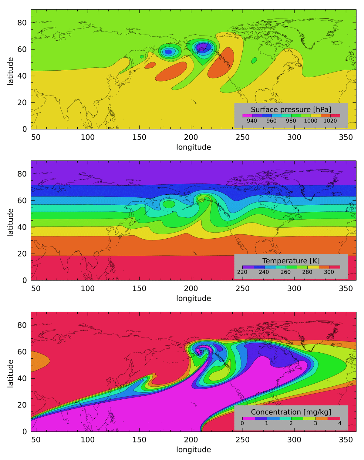
Figure 1
Representative fields from the evolution of the baroclinically-unstable wave at t = 9 days. The surface pressure (top) and temperature on the 850 mb surface (middle) are directly comparable to other model results in Jablonowski and Williamson (2006). The idealized passive tracer on the 500 mb surface (bottom) is initially zero in the sunlit regions of the globe; it illustrates the representation of three-dimensional transport in NEPTUNE.
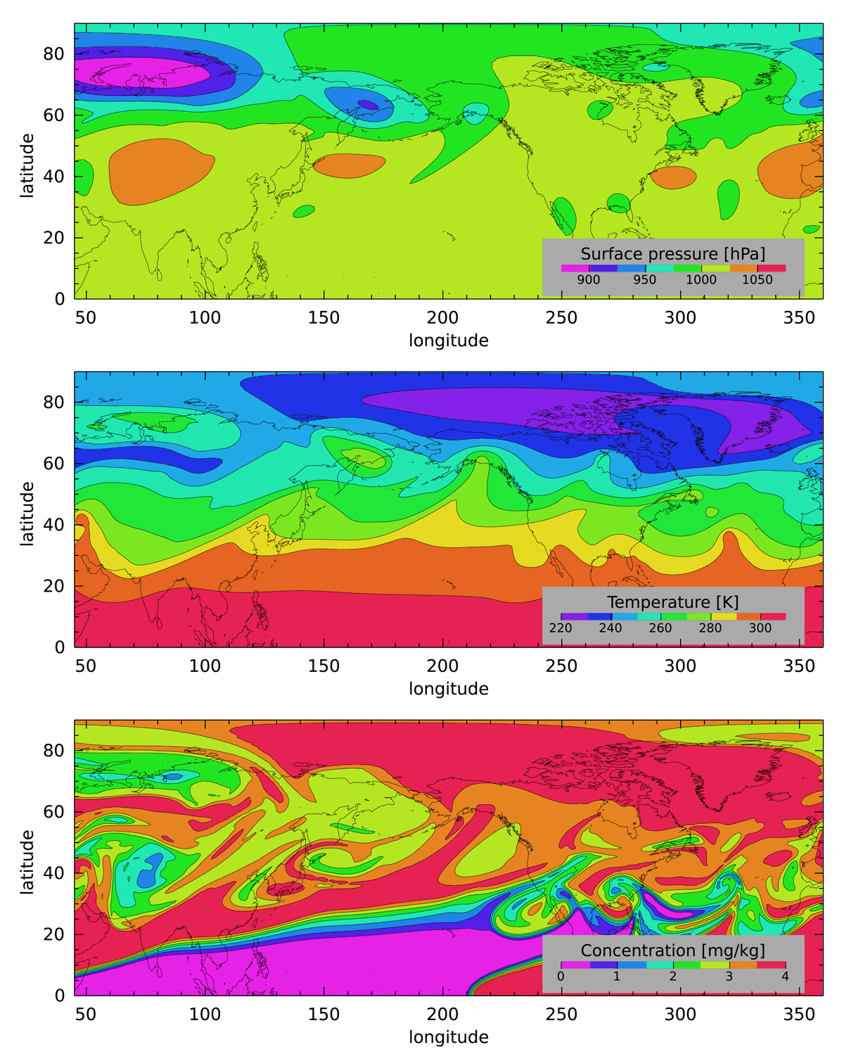
Figure 2
Representative fields from the evolution of the baroclinically-unstable wave at t = 18 days. The pressure (top) and temperature (middle) fields appear to be a mixture of wave-like and eddy-like disturbances. The tracer field (bottom) is undergoing vigorous chaotic stirring.
During time period shown, the baroclinic instability evolves into a strongly nonlinear state in which eddys pinch off from the initially wave-like disturbance. By day 18, the midlatitude flow consists of large-amplitude disturbances on the initial zonally-symmetric pressure and temperature fields. The tracer field has been stirred extensively and appears to be in a chaotic state. The strong vertical shear, coupled with vertical transport, is responsible for the isolated “islands” of tracer concentration between its initial extreme values.
4.1 TLM approximation of finite-amplitude perturbation growth
Numerical experiments were conducted to assess the stability of the TLM linearized around representative time-dependent background states. The purpose of these experiments is to assess the significance of the simplified vertically-implicit solver in the TLM as compared with the complete model and to verify that the TLM adequately represents the non-acoustic modes relevant to numerical weather prediction.
Let qb(x, t) denote the NEPTUNE solution of the JW test case, illustrated in Figures 1 and 2. Beginning with the solution at t = 9 days, qb is used to define the background state around which the TLM is linearized. The solution is also used to compute initial conditions which are representative of a model forecast error field, denoted Δ, equal to . The numerical experiments consist of 72-hour integrations of the TLM from day 9 through day 11.
The TLM solution is compared with two solutions of the nonlinear NEPTUNE model initialized with finite-amplitude perturbations of qb(x, t = 9 d) to quantify nonlinearity over the integration window. Let Δ+ denote the difference between NEPTUNE solution initialized from qb(x, t = 9 d) + Δ and the unperturbed solution, qb(x, t); and let Δ– denote the difference between qb(x, t) and the solution initialized with qb(x, t = 9 d) – Δ. The error in the TLM solution relative to the finite-amplitude perturbation will be quantified with Δ+ – Δ, which may be compared with the model’s nonlinearity, Δ+ – Δ– (see Mahfouf 1999).
Figure 3 illustrates the TLM potential temperature at T = 9 hr and T = 24 hr from initial conditions at t = 9 d. The perturbation, Δ, exhibits an evolving annular pattern associated with the baroclinic wave over northern North America. The error of the TLM solution compared to the nonlinear perturbation, Δ+ – Δ, has a peak amplitude of less than half that of Δ. While this error is a relatively large fraction of the perturbation amplitude, it is localized to the region of most intense nonlinearity and it is comparable to the Δ+ – Δ– field. Tests of the TLM at earlier times, when the evolution is more linear, yield correspondingly smaller errors.
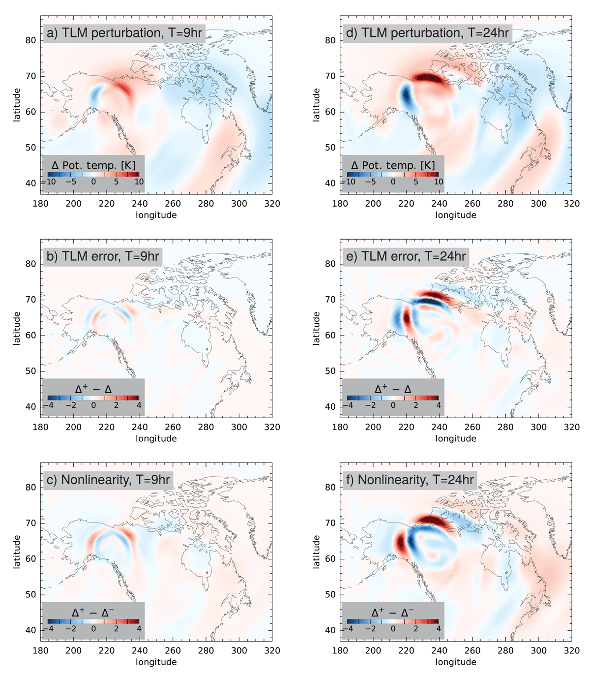
Figure 3
Comparison between the TLM potential temperature and nonlinear perturbation in NEPTUNE. The TLM is initialized with a perturbation equal to 1/8th the difference of the JW baroclinic test case at days 10 and 11, using all NEPTUNE prognostic variables (density, potential temperature, velocity, and tracer). Panels (a)–(c) show, respectively, the TLM field, Δ, the error with respect to the evolution of the NEPTUNE perturbation, Δ+ – Δ, and the nonlinearity metric, Δ+ – Δ–, at T = 9 hr integration, linearized around the JW test case starting at t = 9 day. Panels (d)–(f) show the evolution after T = 24 hr integration.
The evolution of the meridional velocity perturbation is depicted in Figure 4. In contrast to the potential temperature, the velocity exhibits somewhat larger-scale features associated with propagating waves. The TLM error associated with the wave on the eastern flank of North America is very small. Larger TLM errors occur to the northwest in association with the growing baroclinic instability, and their magnitude is smaller than Δ+ – Δ–, as anticipated.
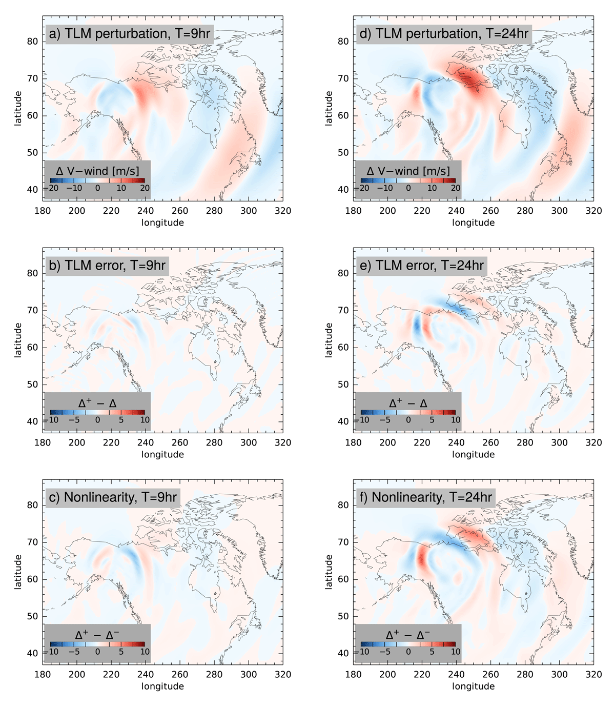
Figure 4
The evolution of a meridional velocity perturbation, as in Figure 3.
Globally averaged root-mean-square (RMS) metrics of the quantities shown in Figures 3 and 4 are compared in Figure 5. Overall, the RMS of Δ and Δ+ closely track one another, and the RMS error, Δ+ – Δ, is smaller than the RMS of Δ until about T = 60 hr. The TLM error increases at about one-half the rate of the nonlinearity metric, Δ+ – Δ–. Of course, the evolution of the error shown here, and its growth rate, depend entirely on the characteristics of the background solution and the initial perturbation. The results demonstrate that the approximate treatment of the acoustic modes in the implicit solver does not create significant limitations for predicting the evolution of perturbations with the TLM.
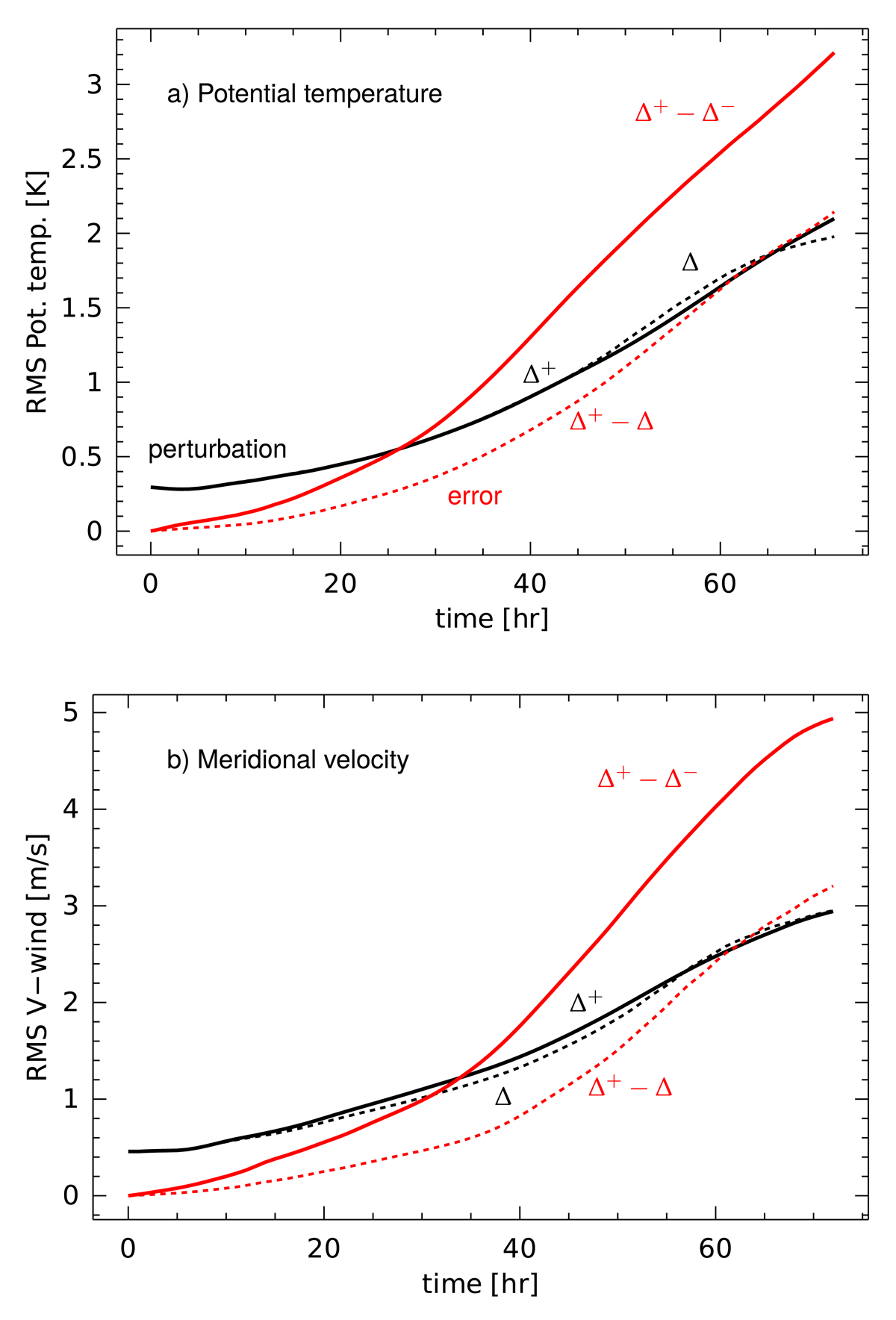
Figure 5
Time series of the root-mean-square (RMS) perturbation solution metrics for (a) potential temperature and (b) meridional velocity. The area-average RMS of the NEPTUNE perturbation solution Δ+ (solid black) and TLM solution Δ nearly overlap throughout the 72-hr integration time. The nonlinearity of the NEPTUNE solution Δ+ – Δ– (solid red) grows at about twice the rate of the error in the TLM solution Δ+ – Δ (dashed red).
4.2 Example of adjoint sensitivity computed with the ADJ
The definition of the adjoint in equation (19) is commonly used within data assimilation algorithms to define a relationship between the value of a measurement of the state at time t = T and the initial conditions at time t = 0. Let p be defined such that d = ⟨p, Lq⟩ is equal to some measurement of interest of the field Lq at t = T, a function of q given at time t = 0. The sensitivity of d with respect to initial conditions q is given by the Jacobian, δd = ⟨L*p, δq⟩. The usefulness of this expression within data assimilation is that, once the field L*p has been computed for a given p, it allows one to compute δd from δq using an inner product, rather than requiring the model to be integrated to evaluate Lδq for all possible δq. Physically, the ADJ is integrated backwards in time, from t = T to t = 0, and evolves the adjoint fields p backwards along time-like characteristics, in duality with the dynamics present in the TLM (Morgan, 2018).
Figure 6 illustrates the evolution in time of the adjoint sensitivity field, p, which corresponds to a measurement of potential temperature at time T = 72 hr on the 850 mb level over North America, linearized around the same background trajectory used in Figures 3 and 4 (the JW test case starting at day 9). The snapshots show how the adjoint potential temperature (Figure 6a–c) is advected backwards by the velocity components of qb. At the earliest time shown, T = 48 hr, which is 24 hr before the measurement (Figure 6c), the sensitivity is dominated by small-scale features associated with instabilities of the background flow. Indeed, comparison with Figure 5 indicates that 24 hr is beyond the limit of useful accuracy of the tangent-linear approximation. The adjoint sensitivity for the meridional velocity component at this level (Figure 6d–f) is driven by a geostrophic adjustment associated with the adjoint temperature at times close to T = 72 hr. At T = 48 hr (Figure 6f) the features in the adjoint sensitivity are dominated by deformations and instabilities of the background flow.
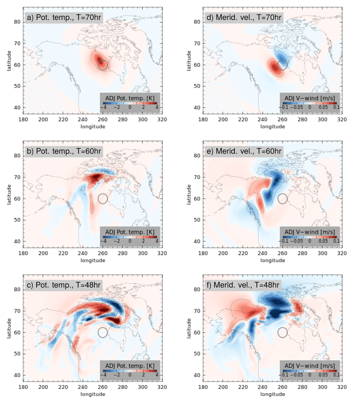
Figure 6
The evolution the adjoint sensitivities on the 850 mb surface for a measurement of potential temperature at T = 72 hr (60∞N, 260∞E, grey circle repeated in each panel). Panels (a)–(c) show the adjoint potential temperature sensitivity, which is predominantly advected backwards towards the northwest along the path of the mean flow at (a) T = 70 hr and (b) T = 60 hr. The complex pattern at (c) T = 48 hr exhibits the smaller scales associated with the deformations of the background flow. Panels (d)–(f) show the adjoint sensitivity of the meridional velocity, which is undergoing a geostrophic adjustment with the adjoint potential temperature.
5. Summary
The NEPTUNE model is a solver for the equations of atmospheric motion based on compressible, non-hydrostatic, deep-atmosphere dynamics. The model utilizes Galerkin spectral elements to solve the equations on a cubed sphere grid and is being developed by the U.S. Navy as the core of a new weather prediction system. The advantages of this formulation are primarily connected with the near-ideal scalability of the code on massively parallel systems, which is enabled the balance between intensive element-wise computations and element-to-element communications.
Tangent-linear (TLM) and adjoint (ADJ) models have been developed for the dry dynamical core of the NEPTUNE model, closely following the computational strategies of NEPTUNE. The TLM enables prediction of the linear evolution of increments around a given time-and space-dependent background flow, and the ADJ provides backwards sensitivities of the increments to previous states. Together, these provide two components of a 4D-Var initialization system for NEPTUNE. The other components of such a system include an estimate of the background error covariance, and observational data sets for assimilation, which are currently being adapted from those utilized in the operational NAVGEM system (Hogan et al., 2014).
The results shown demonstrate the accuracy of the TLM and representative ADJ solutions in the context of a standard test case for dry nonlinear baroclinic instability (Jablonowski and Williamson, 2006). Ongoing work with the system involves development of simplified linear and adjoint models for the moist physical parameterizations used in NEPTUNE, based on the Community Column Physics Package (Firl et al., 2021), as well as TLM and ADJ models for NEPTUNE on regional domains.
Data Accessibility Statement
Source code for the NEPTUNE tangent-linear and adjoint modeling system is available for authorized U.S. Navy and Department of Defense collaborators; to obtain access, contact Dr. Alex Reinecke, alex.reinecke@nrlmry.navy.mil, referencing this paper.
Acknowledgements
This project was funded by Office of Naval Research award number N0001422WX00918.
Competing Interests
The authors have no competing interests to declare.