
Table 1
Selected recent heavy rainfall events based on the JMA reports. Start date and end date indicate the start and end dates of each event. Term is the total number of days each event lasted. Hindcast time is equal to the sum of the lead time and term of each event. Type indicates the main cause of heavy rainfall identified in the JMA reports.
| YEAR | START DATE | END DATE | TERM (DAYS) | HINDCAST TIME (DAYS) | TYPE |
|---|---|---|---|---|---|
| 2010 | Jul 10 | Jul 16 | 7 | 8–11 | Baiu front |
| 2016 | Jun 19 | Jun 30 | 12 | 13–16 | Baiu front |
| 2021 | Aug 11 | Aug 19 | 9 | 10–13 | Stationary front |
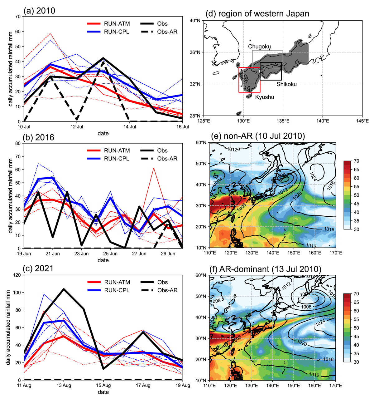
Figure 1
(a), (b), (c): Time variation of daily accumulated rainfall averaged over western Japan during the term of each heavy rainfall event. The thick lines for each case represent ensemble means of each member. The thin solid, dashed, dash-dot, and dotted lines represent 1, 2, 3, and 4 day lead time hindcasts, respectively. The reference reanalysis data (denoted as Obs) were obtained from MSM. Obs-AR represents accumulated rainfall that is related to AR activity. (d): Region of western Japan (land area west of 138°E in the grey shaded region) where the accumulated rainfall was averaged. Kyushu, Shikoku, and Chugoku areas are marked by red, black, and grey colored boxes, respectively. (e), (f): Daily mean column-integrated water vapor (shading, kg m–2) and sea level pressure (contour, hPa) from ERA5 for non-AR case (10 Jul) and AR-dominant case (13 Jul) in 2010.
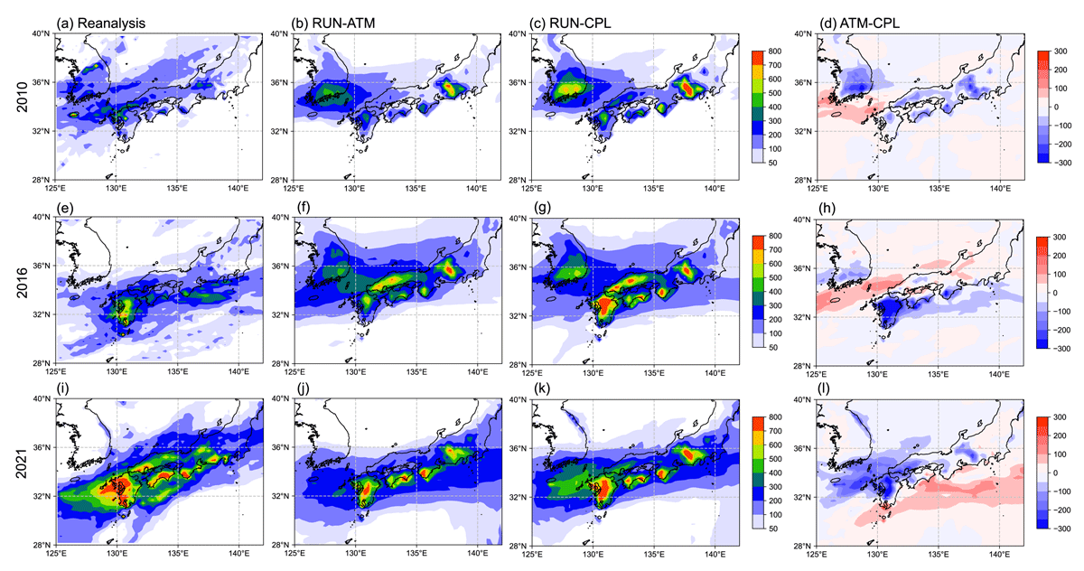
Figure 2
Distributions of accumulated rainfall (mm) during the term of each heavy rainfall event. (a), (e), (i): Reanalysis (MSM), (b), (f), (j): accumulated rainfall in RUN-ATM, (c), (g), (k): accumulated rainfall in RUN-CPL, and (d), (h), (l): differences of accumulated rainfall between RUN-ATM and RUN-CPL. Hindcast results are given as ensemble means, and the ensemble means were computed using hindcast with 1–2 day lead time. Each row represents a different heavy rainfall event.
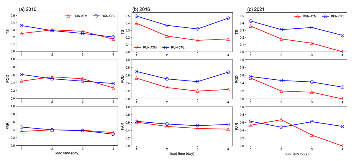
Figure 3
Threat score (TS), probability of detection (POD), and false alarm rate (FAR) of hindcast experiments for heavy rainfall over Kyushu area. Each score is calculated for heavy rainfall exceeding 5 mm h–1 in (a) 2010 and (b) 2016, and heavy rainfall exceeding 10 mm h–1 in 2021. Note that weaker rainfall intensity was used for 2010 and 2016 events, since the rainfall intensity of these cases were weaker than that of 2021 event. The 3-hourly rainfall data from the reanalysis and hindcast experiments were used to compute the statistical values.
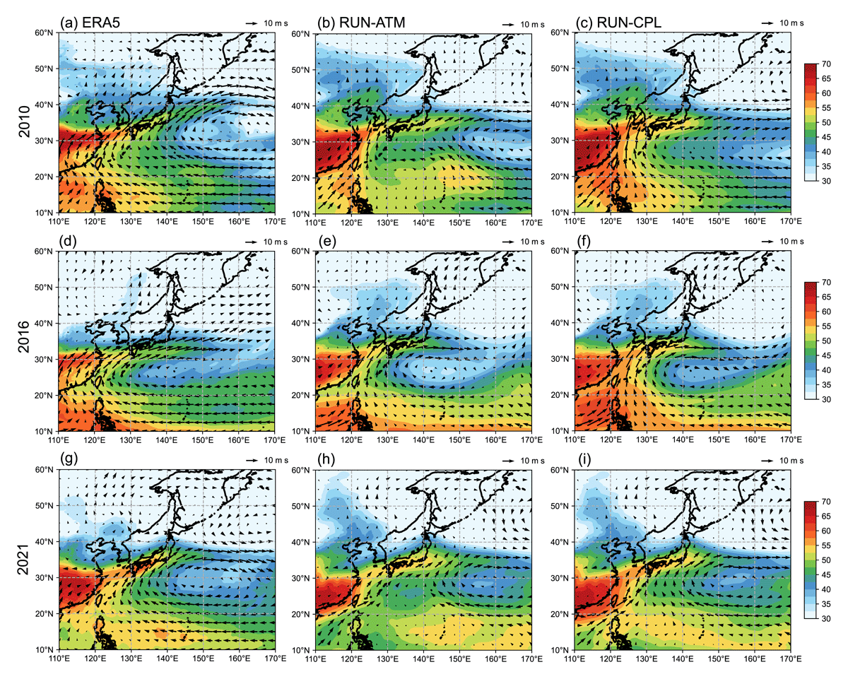
Figure 4
Distributions of IWV during the heavy rainfall events. The shading and vectors indicate IWV (kg m–2) and wind velocity at 850 hPa level (m s–1), respectively. IWV and wind velocity are time-averaged across the term of each event, and the hindcast results are presented by averaging ensemble means of hindcast with 1–4 day lead time. The first, second, and third columns respectively represent the reanalysis (ERA5), RUN-ATM, and RUN-CPL, and each row represents a different heavy rainfall event.
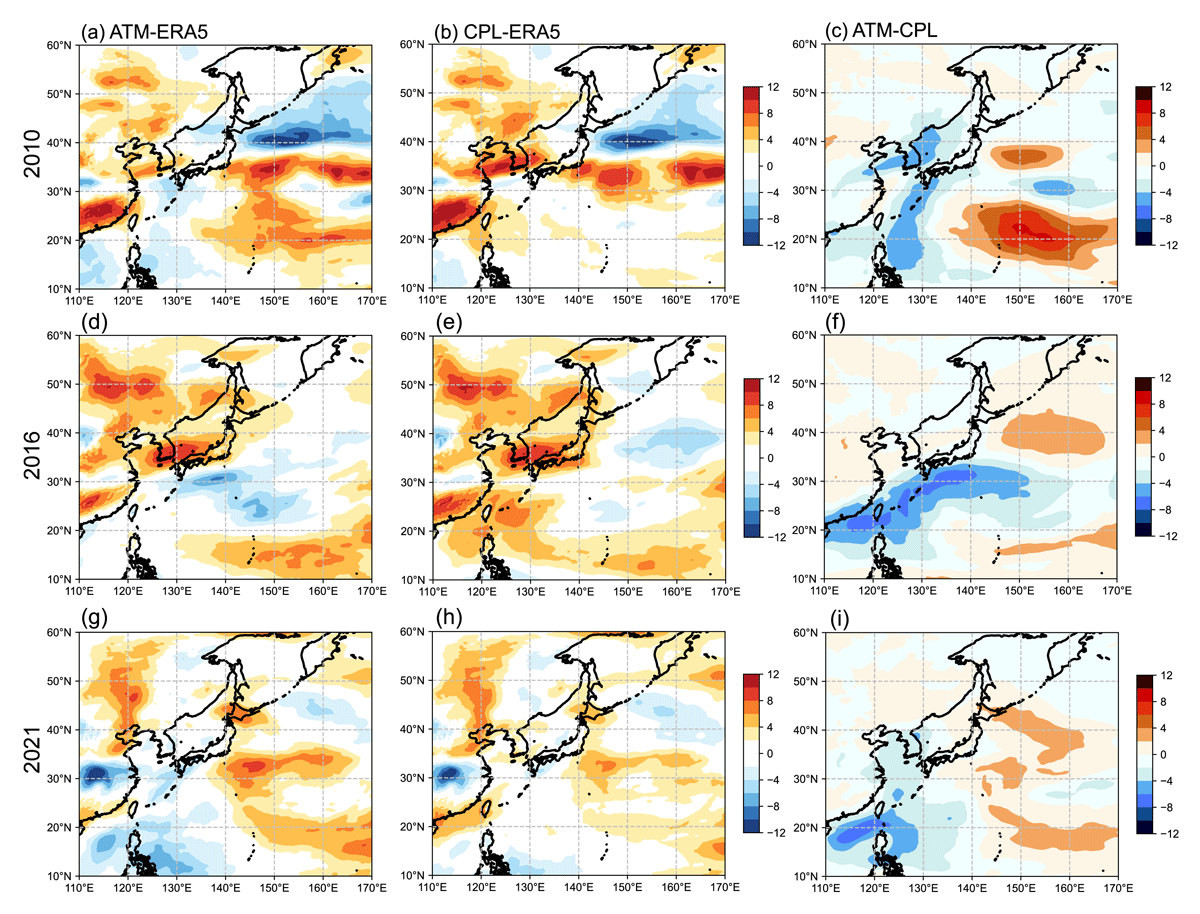
Figure 5
Distributions of difference in the time-averaged IWV (kg m–2) shown in Figure 4. (a), (d), (g): Difference in the IWV between RUN-ATM and ERA5, (b), (e), (h): difference in the IWV between RUN-CPL and ERA5, and (c), (f), (i): difference in the IWV between RUN-ATM and RUN-CTL.
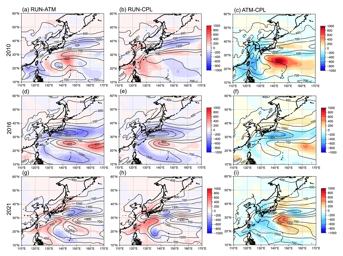
Figure 6
Distributions of IVT (kg m–1 s–1) during each heavy rainfall event by the lead time and cases. (a), (b), (d), (e), (g), (h): IVT (contour line) is for each case (mean of 3–4 day lead time), the IVT differences (shading) were calculated as the mean of 3–4 day minus the mean of 1–2 day lead time, and (c), (f), (i): IVT predicted by RUN-CPL (contour line, mean of 1–2 day lead time), and IVT differences calculated from RUN-ATM minus RUN-CPL (shading, mean of 1–2 day lead time).
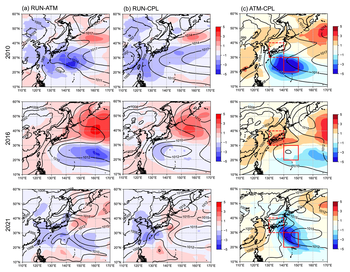
Figure 7
As Figure 6 but for sea level pressure (hPa). Red colored solid box and red colored dashed box indicate area A (140°–150°E and 20°–30°N) and area B (130°–140°E and 30°–40°N), respectively.
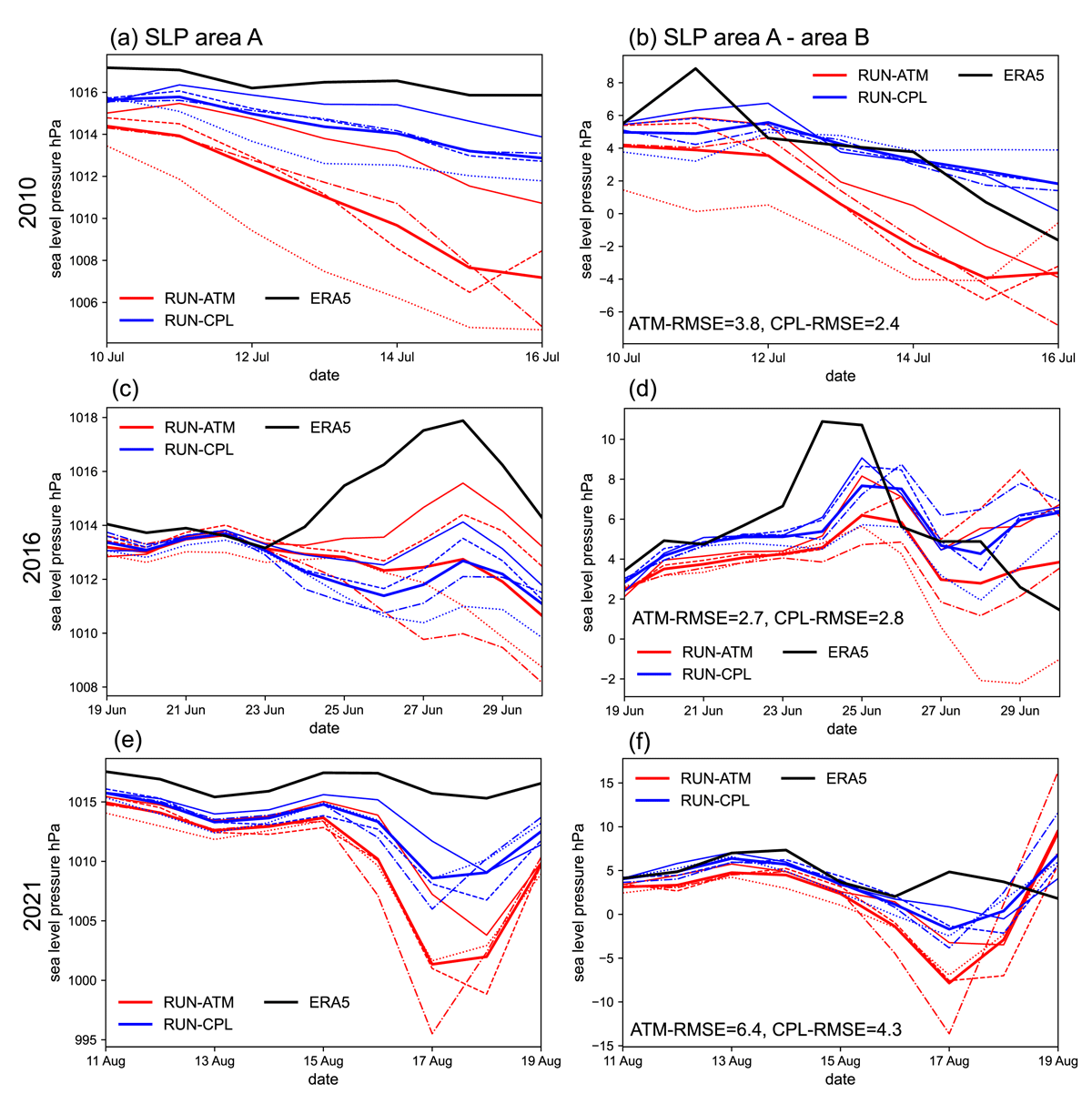
Figure 8
Time variations of area-averaged SLP and SLP difference for each heavy rainfall event. (a), (c), (e): Time variation of SLP averaged for area A. (b), (d), (f): Time variations of SLP difference between area A and area B. The solid, dashed, dash-dot, and dotted lines represent hindcast of 1, 2, 3, and 4 day lead time, respectively. Each row corresponds to a different heavy rainfall event. ATM-RMSE and CPL-RMSE in the right column figures represent root-mean-square error of SLP difference for each hindcast case compared with the SLP difference of ERA5.
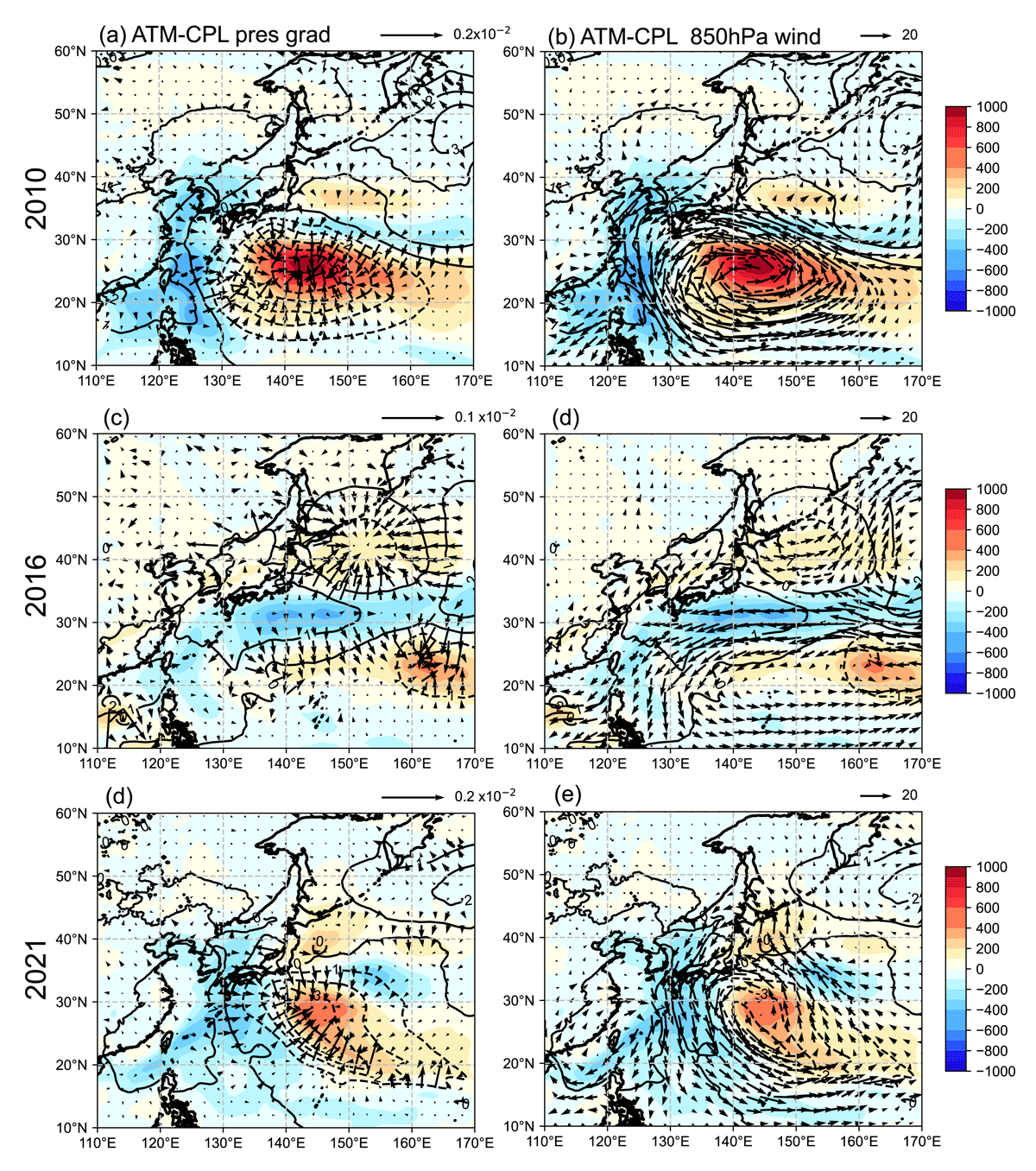
Figure 9
Comparison of SLP difference (contour line, hPa, 1 hPa interval), and IVT difference (shading, kg m–1 s–1), pressure gradient force (vector in left column, Pa m–1) estimated from the SLP difference, and horizontal wind difference at 850 hPa (vector in right column, m s–1). Differences in SLP and IVT are defined by RUN-ATM minus RUN-CPL, and are common for left and right column figures. Results of time-averaged hindcast of 1–2 day lead time during the each event are used to compute the differences.
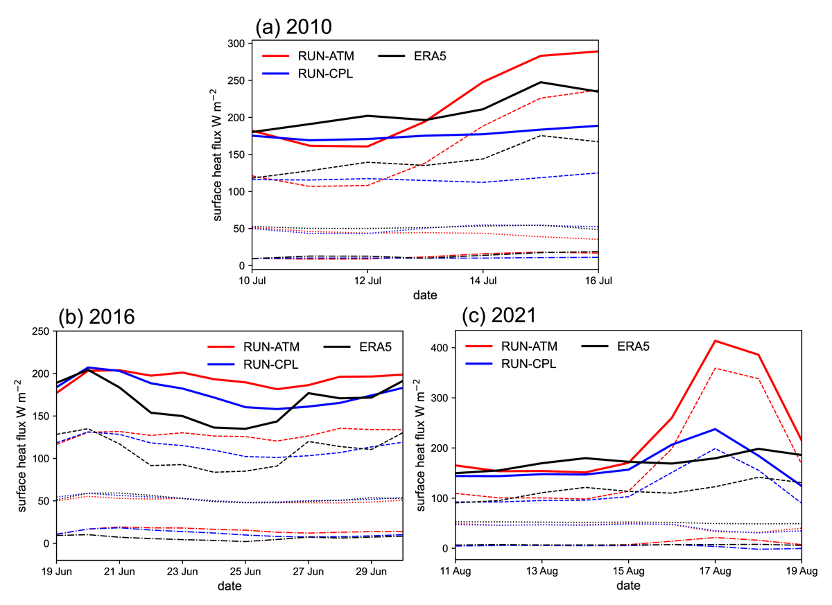
Figure 10
Time variation of various area-averaged surface heat fluxes. The solid, dashed, dash-dot, and dotted lines represent total heat flux, latent heat flux, sensible heat flux, and surface net thermal radiation, respectively. The surface heat fluxes are area-averaged for the area A and are given by the means of hindcast with 1–4 day lead time.
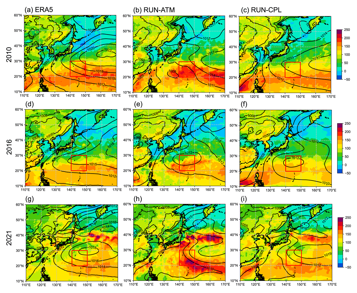
Figure 11
Distributions of time-averaged latent heat flux (shading, W m–2) and SLP (contour lines, hPa). Each variable was time-averaged over the term of each event, and the hindcast is given by the means of hindcast with 1–4 day lead time. The first, second, and third columns respectively represent the distributions of reanalysis (ERA5), RUN-ATM, and RUN-CPL, and each row represents a different heavy rainfall event. The region of area A is marked by red colored boxes.
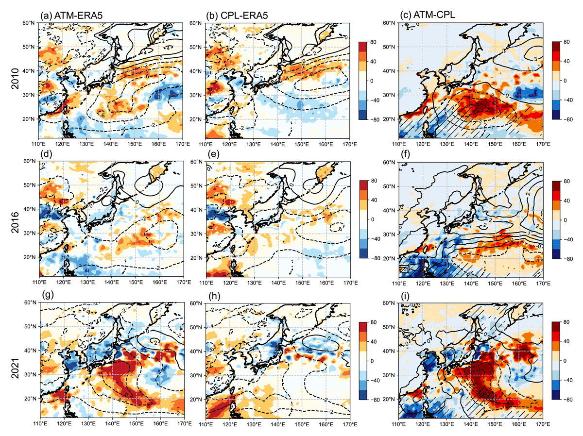
Figure 12
(a), (d), (g): Differences in the latent heat flux (shading, W m–2) and SLP (contour lines, hPa) between RUN-ATM and ERA5. (b), (e), (h): As (a), (d), (g) but for differences between RUN-CPL and ERA5. (c), (f), (i): As (a), (d), (g) but for differences between RUN-ATM and RUN-CPL. The hatching indicates the region where the prescribed SST decreased from the start date of the hindcast for RUN-ATM prediction.
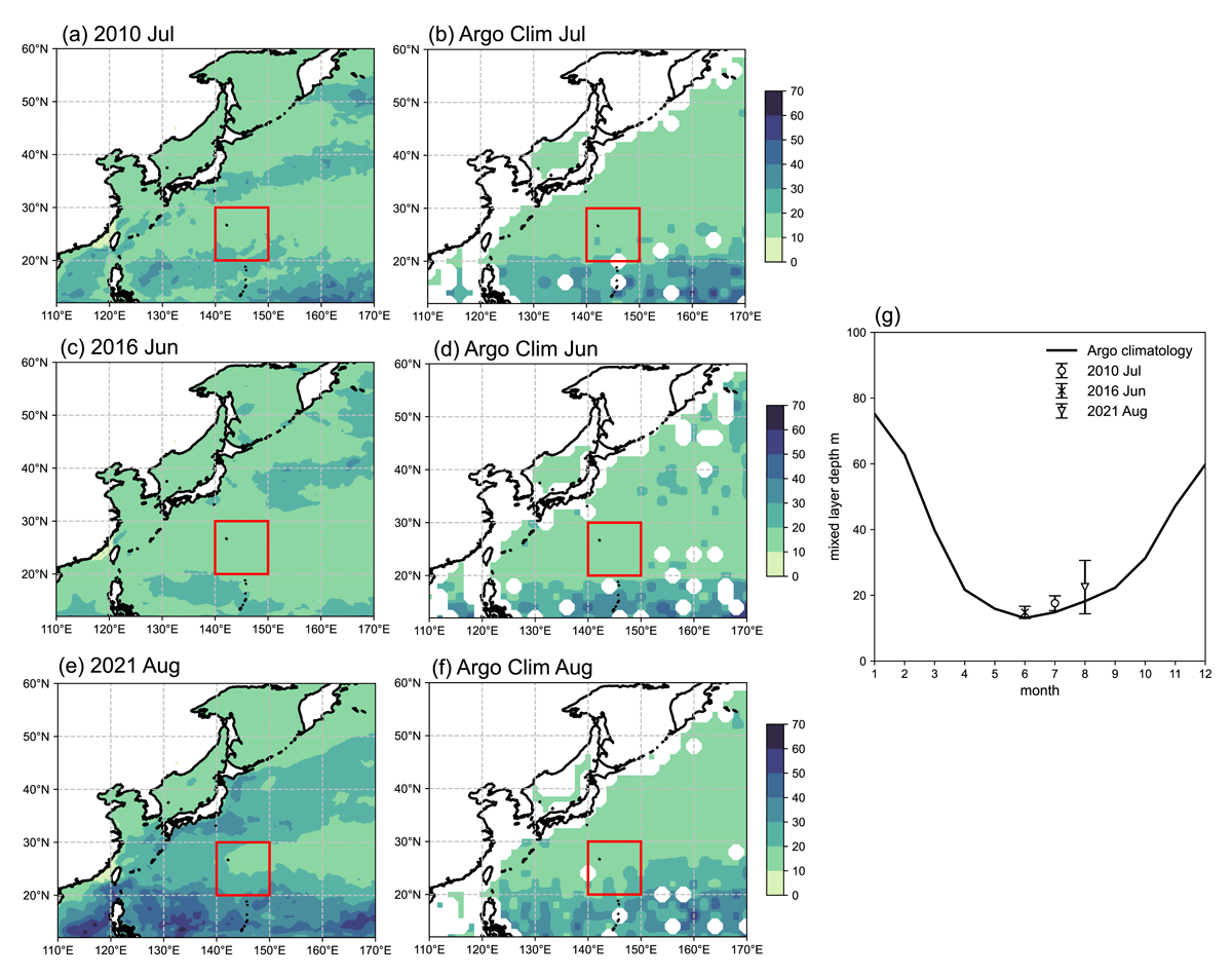
Figure 13
Time-averaged distributions of predicted MLD (m) in the heavy rainfall events with the corresponding observed climatological MLD. (a): RUN-CPL in Jul 2010, (b): Argo Jul climatology, (c): RUN-CPL in Jun 2016, (d): Argo Jun climatology, (e): RUN-CPL in Aug 2021, and (f): Argo Aug climatology. (g): Comparison of area-averaged (area A, marked by red colored boxes) MLD and climatological MLD (the error bars represent 1.5 standard deviations). The MLD distributions are time-averaged for the term of each event. Argo-derived observational data (Hosoda et al. 2010) were used as the reference.
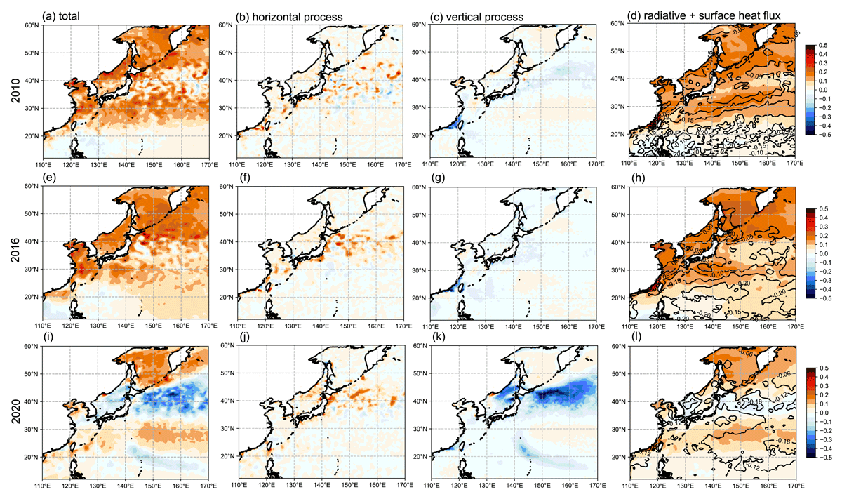
Figure 14
Distributions of ML temperature tendencies (C° day–1) averaged during each heavy rainfall event, obtained from the ensemble mean of hindcast with 1–4 day lead time. (a), (e), (i): Total tendency, (b), (f), (j): tendency by horizontal processes, (c), (g), (k): tendency by vertical processes, and (d), (h), (l): tendency by radiative and surface heat fluxes (shading: all fluxes; contour lines: sum of tendencies by outgoing fluxes including longwave radiation, sensible and latent heat fluxes). Each row corresponds to the tendency of each event time-averaged over the term.