
Global carbon cycle science essentially started in 1958, when Charles (Dave) Keeling began measuring carbon dioxide (CO2) concentrations, first at Mauna Loa in Hawaii and then at the South Pole (Keeling, 1960). Keeling rapidly identified the clear seasonal cycle, with atmospheric CO2 concentrations reaching a minimum in summer and a maximum in winter, and also recorded the clear upward trend in atmospheric CO2 concentration over the years (Keeling, 1960; Keeling, 1970). He immediately attributed this long-term increase to human activities, writing in his 1960 Tellus paper: ‘At the South Pole the observed rate of increase is nearly that to be expected from the combustion of fossil fuel’ (Keeling, 1960). After more than 60 years of continuous measurements, atmospheric CO2 continues to increase year after year, now being more than 100 ppm higher than when Keeling initiated these measurements in 1958 (Friedlingstein et al., 2026). Keeling further showed that about half of the CO2 produced by the combustion of fossil fuels remained in the atmosphere (in Howe & Sutter, 1963; Keeling, 1970; Keeling, 1973; Keeling et al., 1976). Doing so, Keeling implicitly described the airborne fraction, the fraction of anthropogenic CO2 emissions that remains in the atmosphere (Figure 1). The fate of fossil CO2 emissions had been discussed before (Bolin & Eriksson, 1959; Callendar, 1938; Callendar, 1958; Revelle & Suess, 1957) but with the estimate of the airborne fraction essentially ranging between 0 and 1, lacking enough observational evidence of the atmospheric CO2 increase.
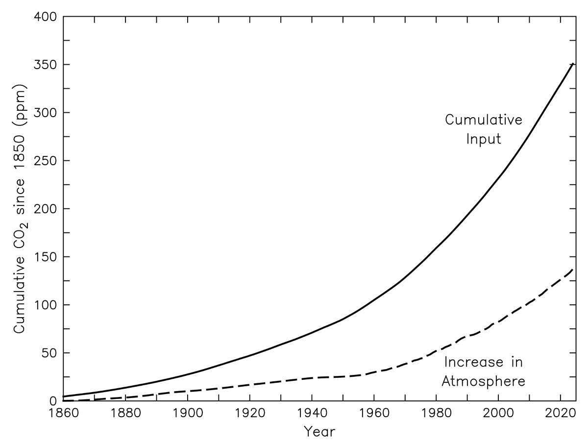
Figure 1
An estimate of the input of anthropogenic CO2 into the atmosphere and the increase of atmospheric CO2 since the mid-nineteenth century; units are in ppm. Updated from Keeling (1970).
At the time Keeling identified the airborne fraction to be about 50%, it was not clear what was the fate of the other half of the CO2 emissions, but based on relatively simple box-diffusion models of the global ocean carbon cycle, the ocean was assumed to be the main sink of anthropogenic carbon, removing about 40% of fossil emissions, with a very small contribution—around 10% at best—from the land biosphere (Broecker et al., 1979; Oeschger et al., 1975).
Additionally, historical land use and land cover change adds CO2 to the atmosphere. This was first hypothesized by Bolin (1977) and Woodwell et al. (1978) and then further confirmed by the work of Richard (Skee) Houghton, who demonstrated that in addition to fossil fuel burning, the land was also a source of CO2 to the atmosphere, primarily via tropical deforestation (Houghton et al., 1983, 1987; Woodwell et al., 1983).
The carbon cycle community realized there was a gap in our understanding of the global carbon cycle, which was called the ‘unaccounted sink’ or the ‘missing sink’ for more than a decade (Broecker et al., 1979; Wigley, 1993). A landmark study published in 1990 by Peter Tans, Inez Fung, and Taro Takahashi provided the first compelling evidence for the existence of a ‘missing’ CO2 sink in the Northern Hemisphere, largely attributable to terrestrial biosphere (Tans et al., 1990). The authors examined the interhemispheric gradient in atmospheric CO2 concentrations between the South Pole and the North Pole. They compared the observed atmospheric measurements with model simulations that incorporated the then well-characterized spatial distribution of anthropogenic CO2 emissions—predominantly concentrated in the Northern Hemisphere—as well as the best available estimates of the oceanic CO2 sink. The simulated interhemispheric CO2 gradient substantially exceeded the gradient derived from atmospheric observations. This discrepancy implied the presence of an additional, unaccounted-for carbon sink in the Northern Hemisphere, the most plausible explanation being a substantial terrestrial carbon sink associated with continental biospheric processes, including enhanced carbon uptake by temperate and boreal ecosystems. This finding marked a pivotal development in carbon cycle science, fundamentally reshaping the understanding of the global carbon budget and highlighting the critical role of Northern Hemisphere terrestrial ecosystems in modulating atmospheric CO2 concentrations. It is worth noting that the finding of Tans et al. (1990) was slightly revised about 15 years later, when atmospheric inversions pointed to a weaker Northern Hemisphere sink and a larger tropical sink (Stephens et al., 2007). The partitioning of the land sink between the tropics and the extra-tropics is still not fully resolved, with atmospheric inversions (top-down) suggesting a larger fraction of the sink in the extra-tropics when compared to land carbon models (bottom-up) (Friedlingstein et al., 2026).
The existence of this ‘missing’ carbon sink was further acknowledged in the First Assessment Report (AR1) published by the Intergovernmental Panel on Climate Change (IPCC) in 1990 (IPCC, 1990). The IPCC report provided a quantitative evaluation of the global carbon budget for the decade 1980–1989, synthesizing the best available estimates of sources and sinks at that time. Anthropogenic emissions from fossil fuel combustion were estimated at approximately 5.4 ± 0.5 GtCyr–1, while emissions associated with land-use change, primarily deforestation, were assessed at about 1.6 ± 1.0 GtCyr–1. Together, these sources amounted to a total annual input of roughly 7.0 GtCyr–1. Atmospheric observations indicated a mean annual increase of approximately 3.4 ± 0.2 GtCyr–1, while the oceanic carbon sink was estimated to account for about 2.0 ± 0.8 GtCyr–1 (Table 1, with the updated global carbon budget for present-day). The IPCC (1990) budget left a large ‘net imbalance’ of 1.6 ± 1.4 GtCyr–1, assessing that:
The result from this budget and from other studies is that the estimated emissions exceed the sum of atmospheric increase plus model-calculated oceanic uptake by a significant amount. The question therefore arises whether an important mechanism has been overlooked. All attempts to identify such a missing sink in the ocean have however failed so far. … There are possible processes on land which could account for the missing CO2 (but it has not been possible to verify them).
Table 1
Global carbon budget in 1990, when the first IPCC report was published (IPCC, 1990), and now, in the latest global carbon budget report (Friedlingstein et al., 2026). All values are decadal averaged, in GtCyr–1. Fractions of total emissions are also shown (in %).
| 1980–1989 | FRACTION (%) | 2015–2024 | FRACTION (%) | |
|---|---|---|---|---|
| Fossil emissions | 5.4 ± 0.5 | 77 ± 14 | 9.8 ± 0.5 | 88 ± 8 |
| Land use change emissions | 1.6 ± 1.0 | 23 ± 15 | 1.4 ± 0.7 | 13 ± 6 |
| Accumulation in the atmosphere | 3.4 ± 0.2 | 49 ± 8 | 5.6 ± 0.02 | 50 ± 4 |
| Uptake by the ocean | 2.0 ± 0.8 | 29 ± 8 | 3.2 ± 0.4 | 29 ± 4 |
| Uptake by the land | 1.6 ± 1.4 | 23 ± 20 | 2.4 ± 0.8 | 21 ± 7 |
Hence, there was a strong suspicion that there was a substantial terrestrial carbon uptake, not captured by inventories or process understanding. Supported by the work of Tans et al. (1990) and other similar studies (e.g., Enting & Mansbridge, 1989; Keeling et al., 1989), the IPCC report therefore acknowledged the significant possibility of a substantial, yet insufficiently quantified, net carbon uptake by the terrestrial biosphere, particularly in the Northern Hemisphere. This conclusion reinforced the emerging view that land ecosystems played a critical and previously underestimated role in regulating atmospheric CO2 concentrations, while also highlighting major uncertainties in carbon cycle quantification at the time.
The 1980s and 1990s saw the development of numerous observational evidence pointing to an accumulation of carbon in the vegetation in response to elevated CO2 (Amthor, 1995; Bazzaz, 1990; Ellsworth et al., 1995; Norby et al., 1999), noting that the actual strength of this fertilization effect is still debated (Canadell & Monteiro, 2021; Walker et al., 2021). In the mid-1990s, new atmospheric oxygen measurements led by Ralph Keeling, combined with the existing atmospheric CO2 measurements, allowed the separation of the land and the ocean sinks, as they have a different oxygen signature, and suggested that the land and ocean carbon sinks had similar magnitude (Keeling et al., 1996).
In parallel, the 1990s saw the development of carbon cycle models, moving from simple box models to spatially explicit process-based models for land (Esser, 1987; Friedlingstein et al., 1995; Melillo et al., 1993; Potter et al., 1993; Rastetter et al., 1991) and ocean (Maier-Reimer & Hasselmann, 1987; Maier-Reimer et al., 1990; Sarmiento & Toggweiler, 1984) carbon cycles. These models were successfully developed and used to help quantify the respective roles of land and ocean to act as carbon sinks over the historical period (Friedlingstein et al., 1995; Kicklighter et al., 1999; McGuire et al., 2001; Orr et al., 2001) or their response to future changes in CO2 and climate (Cramer et al., 2001; Melillo et al., 1995; Prentice et al., 2001; Sarmiento et al., 1998).
These developments proceeded in parallel to developments in climate modeling, from atmosphere-only models to fully coupled atmosphere-ocean-land surface models (e.g., Cubasch et al., 1992; Murphy & Mitchell, 1995; Russell et al., 1995; Washington et al., 1980). Climate models included a representation of the physical ocean and land surface, computing fluxes of water and energy but not yet accounting for the carbon cycle. Climate change simulations were derived from climate models assuming a prescribed change in atmospheric CO2. Until the third IPCC assessment, future climate projections were based on prescribed atmospheric CO2 concentrations rather than on prescribed CO2 emissions. Early experiments were highly idealized, prescribing an immediate doubling of atmospheric CO2 relative to pre-industrial levels (Hansen et al., 1988; Manabe & Stouffer, 1980), and later complemented by transient simulations prescribing a 1% annual increase in CO2 concentrations per year, doubling the concentration in 70 years (Meehl et al., 2000). Those idealized climate model experiments also allowed the quantification of two climate metrics: the Equilibrium Climate Sensitivity (ECS) and the Transient Climate Response (TCR). Subsequently, more policy-relevant concentration pathways—such as the IS92 and Special Report on Emission Scenarios (SRES) scenarios assessed in the Second (AR2) and Third Assessment Reports (AR3) of the IPCC—were adopted (IPCC, 1996, 2001). Crucially, in these simulations, atmospheric CO2 concentrations were specified a priori and used as an external radiative forcing to drive climate simulations; compatible CO2 emissions were derived from these prescribed atmospheric CO2 profiles (Enting et al., 1994; Wigley et al., 1996). Hence, there was no explicit coupling between anthropogenic CO2 emissions and the resulting atmospheric concentrations, as the global carbon cycle was not interactively simulated by these climate models. A central implicit assumption underlying these prescribed atmospheric CO2 experiments was that future climate change would have no impact on the carbon cycle. Future atmospheric CO2 concentrations could be estimated beforehand, from anthropogenic CO2 emissions only. As a result, potential interactions, such as temperature-dependent changes in terrestrial or oceanic carbon uptake, were not represented. This methodological separation between the carbon cycle and the climate system precluded any dynamic feedback between climate change and the processes governing the partitioning of carbon among the atmosphere, ocean, and land biosphere. However, it was known for more than a decade, from ice-core measurements, that there was a strong correlation between atmospheric CO2 and climate, with colder climates (glacial periods) associated with lower atmospheric CO2 concentrations—around 200 ppmv—and warmer climates (interglacial periods) associated with higher atmospheric CO2 concentrations—around 280 ppmv (Barnola et al., 1987; Neftel et al., 1982).
It was not until the late 1990s that fully coupled climate–carbon modeling frameworks were developed. Pioneering work was conducted at the same time in France and the UK, with the development of the IPSL-CM2C and HadCM3LC coupled climate–carbon models (Cox et al., 2000; Friedlingstein et al., 2001). These modeling efforts marked a decisive transition from prescribed-concentration experiments to fully interactive simulations, linking anthropogenic emissions, atmospheric CO2 concentrations, and climate change. In these coupled climate–carbon models, atmospheric CO2 evolved prognostically, as the difference between the prescribed anthropogenic CO2 emissions and the oceanic and terrestrial carbon sinks simulated interactively by the carbon cycle components of the coupled model. The calculated atmospheric CO2 concentrations were then used by the radiative code of the climate to estimate the climate response, as in a traditional global climate model. This framework therefore established a direct and internally consistent link between anthropogenic emissions and the response of the climate system.
Despite differences in the representation of the physical climate system and the land and ocean carbon cycle between the French and British models, their results were qualitatively consistent. Both models identified a positive climate–carbon feedback: climate change reduced the efficiency of natural carbon sinks, thereby amplifying the rise in atmospheric CO2 and reinforcing warming (Friedlingstein et al., 2003). The weakening of carbon uptake was particularly pronounced in the terrestrial biosphere—through mechanisms such as enhanced soil respiration and ecosystem stress—but reductions in oceanic carbon uptake efficiency were also simulated, primarily due to temperature-dependent solubility effects and global oceanic circulation changes. These early coupled simulations provided the first quantitative demonstration that climate change itself could significantly alter the trajectory of atmospheric CO2 concentrations, thereby introducing an additional source of uncertainty and potential amplification in future climate projections.
However, while in agreement on the sign of the climate–carbon cycle feedback, the French and British studies differed significantly on its magnitude. The gain of the climate–carbon cycle feedback, defined as the additional warming simulated in a fully coupled climate–carbon configuration, was estimated to be on the order of 5% for the IPSL-CM2 model and 30% for the HadCM3LC model (Friedlingstein et al., 2003). This large discrepancy, with potentially large implications for the quantification of CO2-induced anthropogenic climate change, led to the rapid development of coupled climate–carbon models in major climate modeling institutions and the establishment of the Coupled Climate–Carbon Cycle Model Intercomparison Project (C4MIP) activity, aiming to quantify the climate–carbon cycle feedback and assess its uncertainty. By 2006, 11 models participated in C4MIP, performing coupled climate and carbon cycle simulations, following the SRES A2 emissions scenario. All participating models consistently simulated a positive climate–carbon feedback, resulting in additional warming relative to uncoupled configurations. However, substantial inter-model spread persisted in the quantification of the feedback strength (Friedlingstein et al., 2006). The dominant source of uncertainty was traced to the terrestrial biosphere. Models differed considerably in their representation of both (i) the sensitivity of land carbon uptake to rising atmospheric CO2 (the so-called β parameter, reflecting the CO2 fertilization effects) and (ii) the sensitivity of terrestrial carbon storage to climate change (the γ parameter, reflecting climate-driven carbon losses) (Friedlingstein et al., 2006).
These findings were formally assessed in the Fourth Assessment Report (AR4) of the IPCC, which, for the first time, explicitly incorporated coupled climate–carbon cycle feedback into its assessment of future climate change (Meehl et al., 2007). The Summary for Policymakers of the IPCC AR4 Working Group I assessed that:
Warming tends to reduce land and ocean uptake of atmospheric carbon dioxide, increasing the fraction of anthropogenic emissions that remains in the atmosphere. For the A2 scenario, for example, the climate-carbon cycle feedback increases the corresponding global average warming at 2100 by more than 1°C. (IPCC, 2007)
In 2009, a series of studies further revealed fundamental properties of the coupled climate–carbon system. First, Solomon and colleagues (2009) demonstrated the irreversibility of anthropogenic CO2-induced climate change on human timescales. Using the BERN-2.5CC model—a coupled climate–carbon cycle model of intermediate complexity—they demonstrate that, even after a complete cessation of CO2 emissions, global temperatures would remain elevated for centuries to millennia. They were the first to explain that this result was due to a near balance between the long-term decrease of radiative forcing due to CO2 concentration decay and reduced cooling through heat loss to the oceans. As a result, atmospheric temperatures would not drop significantly for at least 1,000 years after anthropogenic CO2 emission cease. This finding established that anthropogenic climate change is effectively irreversible on human timescales. This balance between carbon inertia (cooling) and heat inertia (warming) was confirmed a decade later in a model intercomparison study designed to quantify the climate commitment to zero emissions (Jones et al., 2019; MacDougall et al., 2020).
Also in 2009, five papers that were published around the same time analyzed C4MIP simulations and revealed the spectacular near-linear relationship between cumulative CO2 emissions and global mean surface warming (Allen et al., 2009; Gregory et al., 2009; Matthews et al., 2009; Meinshausen et al., 2009; Zickfeld et al., 2009). The linearity was not fully explained but was, again, the outcome of the antagonist effects of the carbon cycle and the climate systems. As warming increases, the efficiency of the carbon cycle reduces because of the positive climate–carbon cycle feedback, leaving a larger fraction of CO2 emissions in the atmosphere, but the radiative forcing of CO2 saturates at a higher CO2 concentration level. These two non-linear responses tend to compensate each other in such a way that cumulative emissions and temperature increase remain approximately proportional over a wide range of CO2 emission levels, and irrespective of the specifics of the emissions scenario. In short, what matters when estimating global warming is the total amount of CO2 emitted to the atmosphere, not its temporality.
This near-linear relationship was hence referred to as the transient climate response to cumulative carbon dioxide emissions (TCRE) and was assessed for the first time in the Fifth Assessment Report (AR5) of the IPCC (IPCC, 2013a). In addition to quantifying TCRE, with a likely range of 0.8°C to 2.5°C warming per 1000 GtC CO2 emitted to the atmosphere, the AR5 made several statements that had profound implications for climate mitigation policies:
A large fraction of anthropogenic climate change resulting from CO2 emissions is irreversible on a multi-century to millennial time scale, except in the case of a large net removal of CO2 from the atmosphere over a sustained period. Surface temperatures will remain approximately constant at elevated levels for many centuries after a complete cessation of net anthropogenic CO2 emissions. (IPCC, 2013b)
Cumulative total emissions of CO2 and global mean surface temperature response are approximately linearly related. Any given level of warming is associated with a range of cumulative CO2 emissions, and therefore, e.g., higher emissions in earlier decades imply lower emissions later. A lower warming target, or a higher likelihood of remaining below a specific warming target, will require lower cumulative CO2 emissions. (IPCC, 2013b)
Note that TCRE only represents the CO2-induced warming. Any warming from non-CO2 agents (CH4, N2O, aerosols, etc.) is not included in TCRE and needs to be accounted for to estimate the overall human-induced warming. However, as CO2 is the main warming agent, the implications for climate policy were very clear: stabilizing global temperature at any chosen level requires reaching zero CO2 emissions. There is essentially no level of long-term CO2 emissions that would be compatible with climate stabilization. This finding was in stark contrast with previous IPCC assessments where the focus was on the stabilization of concentrations, implying non-zero positive CO2 emissions for centuries in the future (Enting et al., 1994; Wigley et al., 1996).
This new scientific understanding of the direct link between cumulative emissions and warming level directly informed international climate policy and was at the core long-term temperature goal of the Paris Agreement at COP21 (UNFCCC, 2015). The Agreement calls:
In order to achieve the long-term temperature goal set out in Article 2, Parties aim to reach global peaking of greenhouse gas emissions as soon as possible, recognizing that peaking will take longer for developing country Parties, and to undertake rapid reductions thereafter in accordance with best available science, so as to achieve a balance between anthropogenic emissions by sources and removals by sinks of greenhouse gases in the second half of this century… (UNFCCC, 2015, Article 4, paragraph 1)
The need to achieve a balance between emissions by sources and removals by sinks was effectively formalizing the requirement of net-zero CO2 emissions to achieve the goal of the Paris Agreement (‘holding the increase in the global average temperature to well below 2°C above pre-industrial levels and pursuing efforts to limit the temperature increase to 1.5°C above pre-industrial levels’). In comparison, the 2009 Copenhagen Accord (UNFCCC, 2009) had much weaker ambitions, only stating:
We agree that deep cuts in global emissions are required according to science, and as documented by the IPCC Fourth Assessment Report with a view to reduce global emissions so as to hold the increase in global temperature below 2 degrees Celsius.
The scientific advances associated with net-zero emission targets also led to the development of the concept of the remaining carbon budget (RCB), defined as the cumulative amount of CO2 that can still be emitted while maintaining a specified probability of limiting global warming below a given temperature threshold (Figure 2) (Friedlingstein et al., 2014; Matthews et al., 2020; Raupach et al., 2014; Rogelj et al., 2016).
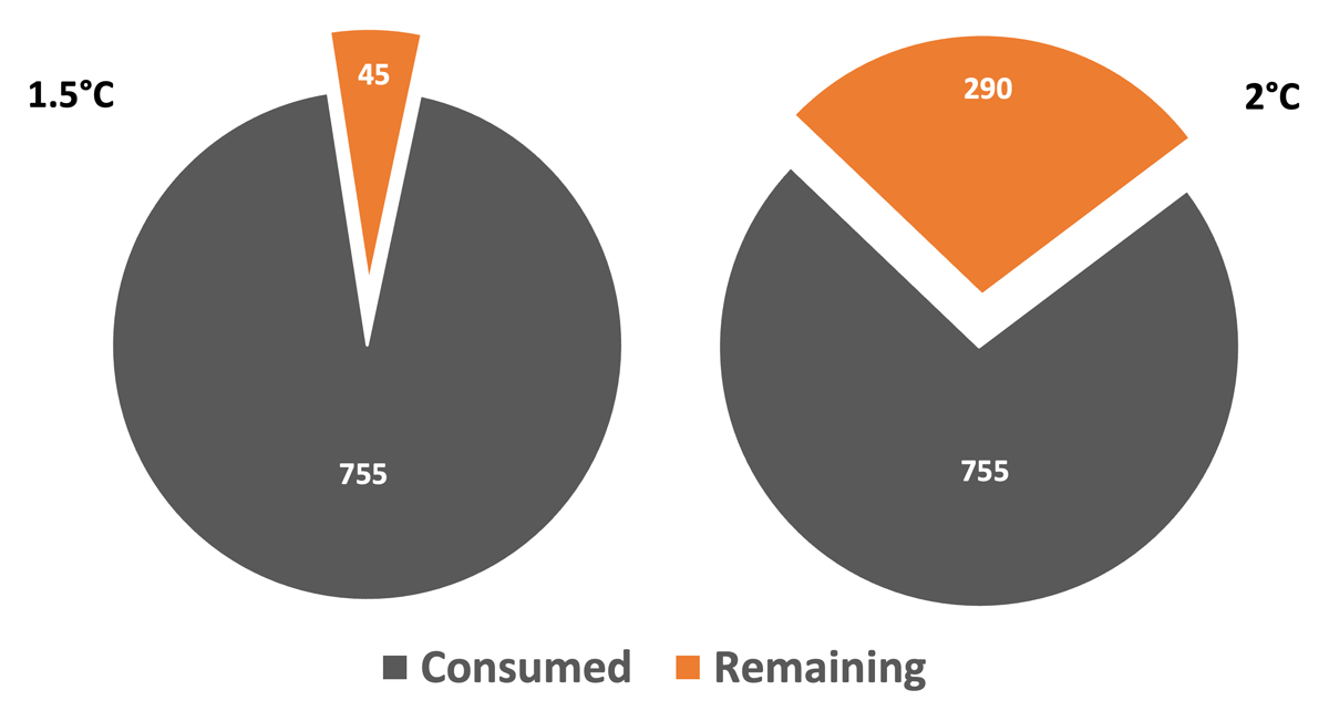
Figure 2
The remaining carbon budget for limiting warming to 1.5°C and 2°C above pre-industrial levels; units are in GtC. Adapted from Friedlingstein et al. (2026).
As assessed in the Sixth Assessment Report (AR6) of the IPCC, for limiting global warming to 1.5°C above pre-industrial levels, the RCB from 2020 was estimated at approximately 140 GtC (500 GtCO2) for a 50% likelihood (IPCC, 2021). For 2°C, the corresponding budget was estimated at 640 GtC (2350 GtCO2). These estimates are subject to substantial uncertainties arising from several factors: (i) the uncertainty in the estimate of TCRE, (ii) the contribution of non-CO2 greenhouse gases to future global surface temperature change, (iii) the zero-emission commitment (the residual warming expected after anthropogenic emissions cease), and (iv) Earth system feedbacks, such as those associated with permafrost or vegetation dynamics that are incompletely represented in current ESM generation and hence in the estimate of TCRE.
Since the publication of AR6 of the IPCC, global CO2 emissions have continued to increase, with current global anthropogenic CO2 emissions from fossil and land use change estimated to have reached 11.5 ± 0.9 GtCyr–1 in 2025 (Friedlingstein et al., 2026), further reducing the remaining carbon budget.
The latest estimate from the global carbon budget, combining the IPCC estimate (IPCC, 2021) and the Indicators of Global Climate Change estimate (Forster et al., 2025), both updated to the year 2026 (i.e., accounting for anthropogenic emissions up to 2025), suggests that the RCB compatible with limiting warming to 1.5°C is now approximately 45 GtC (170 GtCO2), implying that at the current emission rate, only about four years of emissions remain before this budget is exhausted. For the 2°C target, the remaining budget is larger, corresponding to roughly 25 years of emissions at the current level.
These results indicate that achieving net-zero CO2 emissions is essential for limiting long-term warming, consistent with the temperature goals of the Paris Agreement. However, the remaining carbon budget for 1.5°C is virtually gone, meaning that breaching the global surface warming level of 1.5°C is now unavoidable. This admission of failure, despite more than 60 years of rigorous scientific information on human influence on the carbon cycle and the climate system, can only call for a significant reinforcement of global mitigation efforts.
Abbreviations
C4MIP: Coupled Climate–Carbon Cycle Model Intercomparison Project
ECS: Equilibrium Climate Sensitivity
ESM: Earth System Model
IPCC: Intergovernmental Panel on Climate Change
RCB: Remaining Carbon Budget
SRES: Special Report on Emission Scenarios
TCR: Transient Climate Response
TCRE: Transient Climate Response to Cumulative Carbon Dioxide Emissions
UNFCCC: United Nations Framework Convention on Climate Change
Data Accessibility Statement
All global carbon budget data presented here are available via the Integrated Carbon Observation System (ICOS) Carbon Portal, https://doi.org/10.18160/GCP-2025.
Acknowledgements
I am grateful for the support from the CALIPSO (Carbon Loss in Plant Soils and Oceans) project, funded through the generosity of Schmidt Science.