Stommel’s 1961 Tellus Paper on Thermohaline Circulation Stability: Curious Early History and Lasting Legacy

1. Introduction

The first paper investigating multiple equilibria and hence potential instabilities of the thermohaline circulation (THC, Stommel 1961) was published in Tellus in 1961 by Henry Stommel, generally regarded as the most important physical oceanographer ever. Today, this paper is far and away Stommel’s best cited (at this writing, 1226 citations in Web of Science, 1987 citations in Google Scholar), so obviously it is widely considered seminal for the current extensive research on the stability of the Atlantic Meridional Overturning Circulation (AMOC, the term that has since superseded the term THC). A closer look reveals, however, that the history of this paper’s influence is quite chequered. It accumulated a mere eight citations in the first 25 years (Google Scholar, https://tinyurl.com/mfrufujj). Furthermore, the paper that arguably started the ensuing avalanche of THC/AMOC research by showing that THC instability arose also in three-dimensional ocean general circulation models (OGCMs), Frank Bryan’s Nature paper (Bryan, 1986a), based on his PhD thesis in Princeton (Bryan, 1986b), did not cite Stommel’s Tellus paper.

None of the prominent reviews of AMOC or AMOC stability took a closer look at the details of Stommel’s paper’s influence (e.g., Buckley & Marshall, 2016; Ferreira et al., 2018; Johnson et al., 2019; Kuhlbrodt et al., 2007; Weijer et al., 2019). The only account I am aware of is my own informal and very brief review more than 30 years ago as part of winter school proceedings (Marotzke, 1994). It thus appears timely to present a more comprehensive account in this jubilee issue, aided by additional testimonials. Furthermore, I appraise the numerous strengths of Stommel (1961) that underlie its endurance as the original reference for AMOC instability, but also its main weakness. While many elements of this appraisal can be found in the published literature, they are scattered there, whereas I present a coherent account. Furthermore, quite some papers incorrectly attribute findings to Stommel (1961), something I try to correct here. Finally, some elements of the appraisal, to the best of my knowledge, have not previously been published.

2. The Beginnings

Stommel (1961) comprises a single reference, to an Applied Maths monograph, and a three-line abstract: “Free convection between two interconnected reservoirs, due to density differences maintained by heat and salt transfer to the reservoirs, is shown to occur sometimes in two different stable regimes, and may possibly be analogous to certain features of the oceanic circulation” (p. 224). The paper is thus the quintessential bolt out of the blue, without precedent. The oceanographic motivation arises from the observation that the two surface thermohaline fluxes, heat and freshwater, tend to act “contrarily to each other” (Stommel, 1961, p. 224) in their effects on density: Except in the equatorial rain belt, low-latitude surface water gains heat and thus decreases its density, whereas it loses freshwater and thus increases its salinity and density. The opposite ensues at high latitudes.

Explicitly shying away from the oceanographic complexity, Stommel instead considers a system inspired by classical thermodynamical considerations, by placing the system under scrutiny into external reservoirs of heat and substance (salt, Figure 1). Note that in agreement with standard thermodynamical parlance, I call the external constant drivers “reservoirs.” Stommel, unfortunately, uses the term “reservoirs” for the system under consideration itself in the abstract but then switches to “vessels” in the rest of the paper (Figure 1); today we mostly use the term “boxes.” Despite Stommel’s at times self-deprecating language (for instance, “That is all we propose to do here.,” p. 224), it is clear from the paper that he thinks of his boxes as representing the low and high latitudes of the ocean.

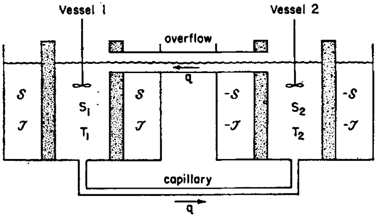
Figure 1

There are two crucial elements of Stommel’s model that lead to interesting behavior. The first is that the forcing for temperature is assumed to occur faster than that for salinity (“we form an impression that the heat transfer mechanism has a more rapid effect on the density of a newly arriving parcel of water,” p. 224). The second is that the flow is proportional to the density difference between the boxes, implying a quadratic nonlinearity in the advection of temperature and salinity (see Section 6). Another nonlinearity enters because the advection term depends only on the magnitude of the flow and not on its direction (see Section 6). These nonlinearities cause the existence of three equilibria under certain parameter settings, two of which, with opposite flow directions, are stable to small perturbations and one of which is unstable. The latter would today be called a tipping point. One stable solution, in which the temperature difference between the boxes dominates the density difference, implies sinking at high latitudes; the other, with the salinity difference dominating, implies sinking at low latitudes. Stommel (1961) finds the equilibria graphically and determines the stability by linearization about the equilibria.

3. The First 30 Years

Stommel (1961) faced an inauspicious beginning. A colleague of his at Harvard University at that time recollects that, in a presentation around 1960, Stommel himself did not emphasize oceanic applicability of his box-and-pipe contraptions (Peter Stone, 1993, personal communication), and the community appears to have largely agreed. The following 25 years were more markedly characterized by who did not cite the paper than by who did. Let us still begin with those who did. Most did so in passing—with one curious exception. Stommel and Rooth (1968) is a mathematically nearly equivalent follow-up to Stommel (1961), with wind as the fast and thermal forcing as the slow antagonist. I will return to this paper shortly.

Stommel (1961) was not cited in any of the 18 review papers comprising the monumental book Evolution of Physical Oceanography (Warren & Wunsch, 1981) that celebrated Stommel’s 60th birthday in 1980—although all authors went out of their way to pay appropriate tribute to Stommel’s outsized contributions to the field. And the paper was not cited in the very influential 1982 paper by Claes Rooth, who presented a box model sharing many similarities with Stommel’s but covering a pole-to-pole circulation within one ocean basin (Rooth, 1982). Most crucially, the flow strength was determined not by the density difference between high and low latitudes but by the density difference between the high northern and the high southern latitudes.

Rooth (1982) focused on the instability of an equatorially symmetric circulation. Furthermore, through frequent visits to Princeton during the early 1980s, Claes Rooth was a major inspiration for Frank Bryan’s thesis work (Claes Rooth, 1993, personal communication; Frank Bryan, 2025, personal communication), which had the maintenance of the interhemispheric THC as one of its two foci (Bryan 1986a; Bryan 1986b). Given the existence of Stommel and Rooth (1968), it seems curious that none of Rooth (1982), Bryan (1986a), and Bryan (1986b) cited Stommel (1961). However, Claes Rooth recollects that when he published his 1982 paper, he was much more influenced by palaeo-oceanographic discussions than by his own earlier work with Stommel (Claes Rooth, 1993, personal communication). Despite this oversight, Stommel’s original paper must have played a role, consciously or unconsciously. Frank Bryan recollects that in presenting his thesis work, he routinely referred to Stommel (1961) on his slides; unfortunately, the documents are lost (Frank Bryan, 2025, personal communication).

Broecker, Peteet, & Rind (1985) and Welander (1986) then were the first to state explicitly the relevance of both Stommel (1961) and Rooth (1982) for understanding the global ocean circulation; together they rejoined the seemingly divergent strands of inquiry. However, it was neither of the two box-model studies of THC instability that attracted a larger part of the research community to the topic, but the demonstration that these phenomena also occurred in OGCMs (Bryan, 1986a; Bryan, 1986b). Crucial for this occurrence was the first-ever employment of mixed boundary conditions for temperature and salinity in an OGCM, in that surface temperature was restored to some prescribed profile on a very short timescale, whereas a fixed freshwater flux was imposed for salinity, with no unphysical restoring to some salinity profile.

The first follow-up with an OGCM was the thesis by Christopher Mead in Southampton (Mead, 1988; a thesis totally unknown today), who extended Bryan (1986a) by adding a second ocean basin connected through a southern circumpolar channel. However, Mead (1988) did not push his model hard enough to effect a transition to another equilibrium; note that Mead (1988) cited Rooth (1982) but not Stommel (1961). Simultaneously, Pierre Welander inspired the beginnings of my own PhD thesis in Kiel (Marotzke, 1990, see Marotzke, 2023). We started from a preprint of Bryan (1986a) and first developed an intermediate-complexity model of the THC that could replicate Bryan’s findings (Marotzke, Welander, & Willebrand, 1988), later to be followed by OGCM studies showing multiple equilibria of both single-hemisphere and idealized global configurations (Marotzke, 1989; Marotzke, 1990; Marotzke & Willebrand, 1991). Guided by Pierre Welander’s knowledge of the literature, all these works cited both Stommel (1961) and Rooth (1982). They were also both cited in the first—somewhat serendipitous—demonstration of multiple THC equilibria with a coupled GCM (Manabe & Stouffer, 1988).

4. Lasting Legacy

Thanks to Pierre Welander theoreticians, and modellers following Bryan (1986a) and Bryan (1986b) paid attention to Stommel (1961). However, other groundbreaking work has gone unnoticed before and after (see, for instance, Eunice Foote’s discovery of the greenhouse effect due to CO₂, Foote 1856), sometimes despite efforts to the contrary, so why did Stommel (1961) receive proper credit eventually? One (pessimistic) answer relies on scientific status, one (optimistic) answer on the lasting legacy of the paper.

It may well be that because of Stommel’s fame, people subsequently went out of their way to cite his contribution to AMOC stability. These social dynamics have been called the Matthew Effect, defined as “the accruing of greater increments of recognition for particular scientific contributions to scientists of considerable repute and the withholding of such recognition from scientists who have not yet made their mark” (Merton, 1968, p. 58).

There is some evidence for this assumption. For illustration, one ironically has to consider the first of the core reasons for the lasting legacy of Stommel (1961). In all papers and models finding multiple THC equilibria, they are caused by the positive salinity-advection feedback (see Weijer et al., 2019 for a recent comprehensive review): A low-salinity anomaly in the deepwater-forming ocean or region leads to THC weakening, which leads to reduced transport of salinity into that region, and the initial anomaly is enhanced. While this feedback also underlies the existence of multiple equilibria in Stommel (1961), the original paper provides no physical interpretation of why the multiple equilibria occur, nor does it discuss the salinity-advection feedback. But papers repeatedly ascribe the identification of this feedback to Stommel (1961) (e.g., Johnson et al., 2019; p. 5386; Kuhlbrodt et al., 2007, p. 22), whereas it was first explicitly formulated in a little-known paper by Gösta Walin (Walin, 1985; ironically citing neither Stommel, 1961 nor Rooth, 1982).

However little physical explanation was given explicitly, Stommel must have known the ingredients necessary for the noteworthy behavior in his model, chief among them the salinity-advection feedback. From the mid-1980s onward, his model has then increasingly been invoked for its interpretive power to understand multiple equilibria across a model hierarchy, including GCMs (e.g., Marotzke, 1990; Weijer et al., 2019). The model itself has, in addition, been used as a simulation tool in a wide variety of applications, such as the THC response to stochastic forcing (e.g., Bryan & Hansen, 1995; Cessi, 1994) and the effect of ocean geometry on the THC (e.g., Huang, Luyten, & Stommel, 1992; Marotzke, 1990; Welander, 1986; Youngs, Ferrari, & Flierl, 2020). This wide applicability and application have been the first core reason for the lasting legacy of Stommel (1961).

The second core reason for the lasting legacy lies in the fact that the Stommel model is a surprisingly good representation of the coupled system of the THC interacting with atmospheric meridional transports. This is surprising because the classical-thermodynamic setting in Figure 1 at first sight bears little resemblance to ocean–atmosphere interactions. Surface heat flux can be reasonably described by the “heat bath” metaphor, and sea surface temperature is then restored to some prescribed profile (e.g., Bretherton, 1982; Haney, 1971). However, the same is not true for the salinity boundary condition. Ocean and atmosphere exchange freshwater, not salt, and the influence of these freshwater exchanges on surface salinity cannot even approximately be represented by the “salt bath” metaphor or a salinity restoring. A much better physics-based approximation to the coupled system is the use of mixed thermohaline boundary conditions, introduced by Bryan (1986a). In their extreme form, the mixed boundary conditions prescribe the surface temperature and a virtual surface salinity flux (e.g., Marotzke, Welander, & Willebrand, 1988).

When this is applied to the Stommel box model, it simplifies considerably and is amenable to analytical solution, both for the equilibria and their perturbations, as first shown by Marotzke (1990), see also Marotzke (2000). But there is more: The Stommel box model in this simplification can be seen as an approximation to the coupled system, combining the THC with meridional atmospheric eddy transports (Marotzke & Stone, 1995; Marotzke, 1996). Remarkably, the bifurcation structure does not change much when the coupling is changed—whatever the formulation, one can always find two stable solutions with opposite flow directions and one unstable solution “in between,” the same structure as correctly anticipated in Stommel (1961). The regime with multiple equilibria vanishes only if horizontal diffusion, mimicking transports by the horizontal gyres, becomes too strong (Longworth, Marotzke, & Stocker, 2005).

The third core reason for the enduring legacy of the Stommel model lies in it being a superb teaching tool for dynamical systems. With the simplifications by Marotzke (1990) and constant forcing, the equilibria can be found exactly; linearization about an equilibrium allows the exact identification of the linear feedbacks; the stability can be graphically illustrated by exact phase-space diagrams or by the model’s Lyapunov potential; even the exact time-dependent solution can be formulated explicitly and offers additional insights. Section 6 demonstrates these features.

Despite all its power, the Stommel model shows one grave weakness—its dynamics. That the flow strength is determined by the density difference between high and low latitudes implies that a breakdown of high-latitude sinking is caused by a reversal of the intra-hemispheric density difference; the low latitudes must show higher density than the high latitudes, and the deep ocean should be filled by highly saline instead of cold water. But all of this is quite unrealistic for the Earth’s ocean (e.g., Bice & Marotzke, 2001), and MOC strength in OGCMs is much better described by the density difference between high northern and high southern latitudes, as first shown by Hughes & Weaver (1994). The simplest AMOC model with reasonable dynamics thus is Rooth (1982) and not Stommel (1961).

5. A Teaching Tool for Dynamical Systems

The preceding section already lists the dynamical-systems aspects that can be illustrated with the Stommel (1961) model; here I give a brief explicit theoretical account of these aspects. The power in this collection lies in the complementary perspectives on stability and instability provided by the various approaches; I argue that it is this complementarity that provides the deepest physical understanding.

The model consists of two well-mixed boxes (1: high-latitude; 2: low-latitude) of equal volume (Figure 2, showing the simplification of Marotzke, 1990; Marotzke, 2000). The flow strength q is related to the density difference between the boxes by a linear law,

where k is a hydraulic constant and α, β are, respectively, the thermal and haline expansion coefficients. If q > 0, there is poleward surface flow because high-latitude density is greater than low-latitude density, and vice versa. The box temperatures are assumed to be imposed by the atmosphere, as is the surface freshwater exchange, expressed through an equivalent surface salinity flux H. The conservation equations governing the system are then only those for salinity,

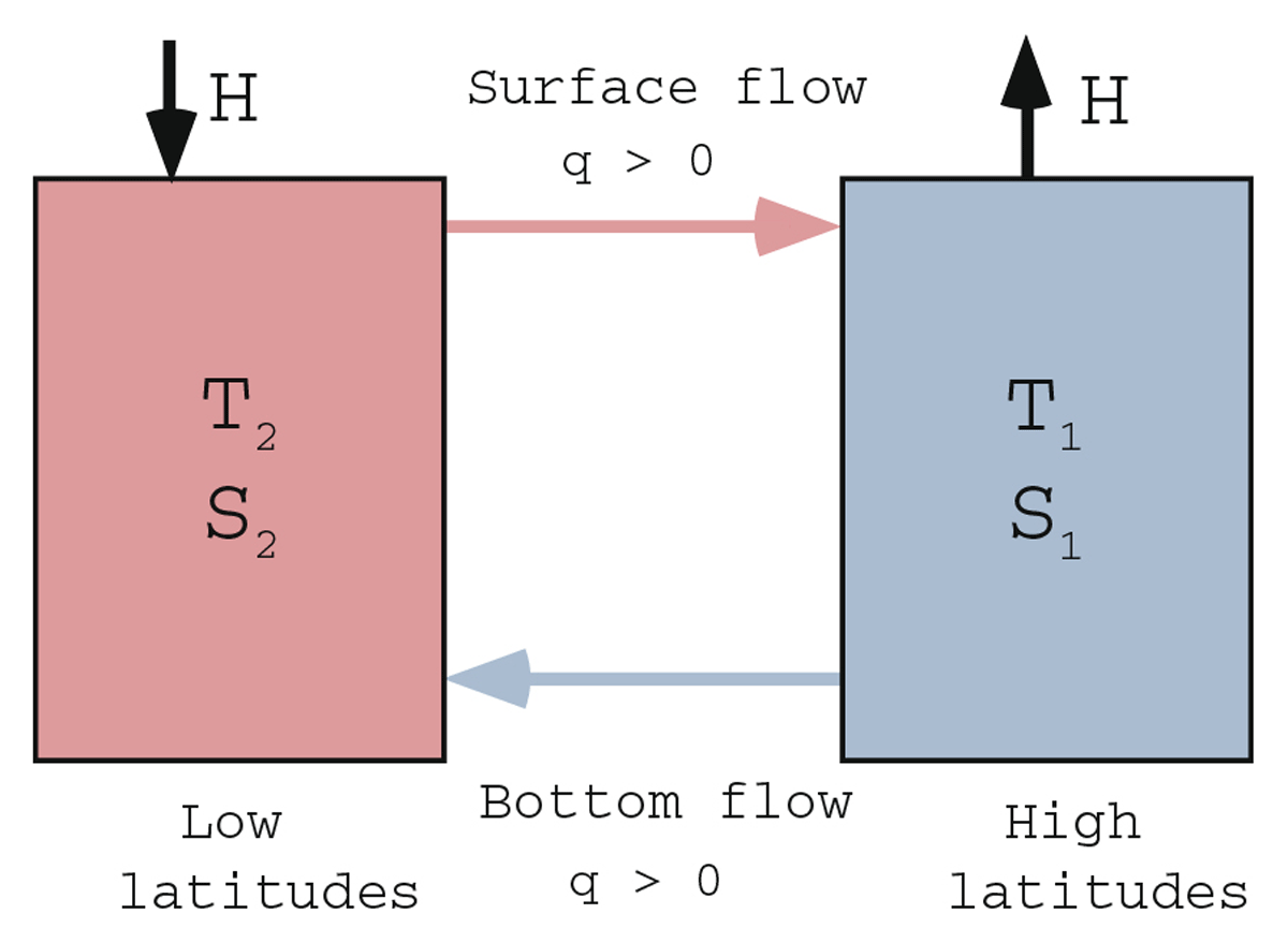
Figure 2

Subtracting (2) from (3) and using (1) leads to

Assuming steady state, marked by an overbar, yields

with solutions

(thermally dominated, poleward near-surface flow) and

(salinity dominated, equatorward near-surface flow; the other root must be discarded). If the radicand in (6) is positive, this simplest possible model of the THC has two stable equilibria, with sinking implied either at high or at low latitudes. A closer inspection shows that it is the combination of nonlinearity and different types of forcing for temperature and salinity that creates the multiple equilibria.

The feedback processes determining stability can be found by linearizing (4) in the vicinity of the equilibria. We write $\Delta S(t)=\Delta \overline{S} + \Delta S^{\prime }(t), \left|\Delta S^{\prime }\right| \ll \Delta \overline{S}$, etc., and find

Using (8) it is readily shown that solution 2 in (6) is unstable to small perturbations and that the instability arises from the salinity-advection feedback, represented by the second term on the right-hand side of (8): An initial positive perturbation in salinity difference weakens the flow, which causes reduced salinity advection, and the salinity difference grows even more. In solution 2 in (6) this positive feedback overwhelms the negative feedback from the mean flow advecting the perturbation in salinity difference (first term on the right-hand side of (8)).

It is useful to nondimensionalise the salinity difference according to

the salinity forcing according to

and time according to

for arbitrary X. We obtain for the time-dependent and steady-state salinity differences

see Figure 3. The phase-space tendencies illustrate that a pair (E, δ) situated to the right of the equilibrium curves has forcing E greater than compatible with equilibrium, and hence a positive phase-space tendency (upward arrow); a pair situated to the left leads to a negative tendency (downward arrow). This allows reading off the behavior of any assumed perturbation from an equilibrium—will it grow or will it shrink?

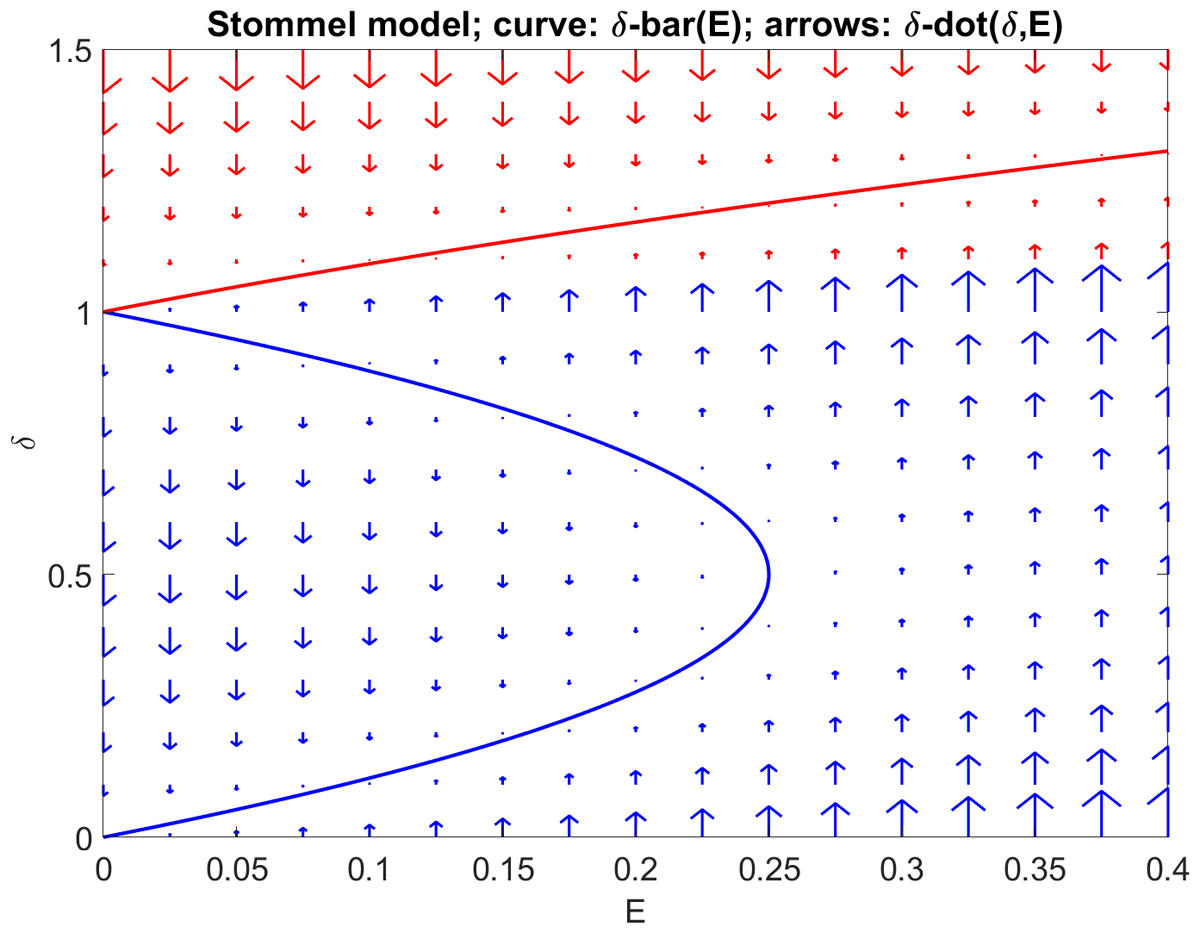
Figure 3

From (12), we infer that the function L defined by

is a Lyapunov potential, the minima and maxima of which define the system’s equilibria. It is readily shown that up to an arbitrary constant, we obtain

and

The minima mark stable equilibria, the maxima unstable equilibria, consistent with the notion of a bead moving on a string under the influence of gravity (Figure 4, note how equilibria arise and vanish as E is varied).

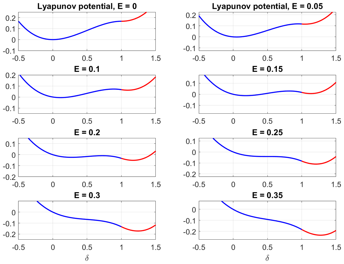
Figure 4

The final illustration concerns the exact time-dependent solution, which, with some algebra, can be verified to be given by

where atanh is the inverse of the hyperbolic tangent tanh, δ(0) is the initial condition, and the expressions are not valid if the initial condition corresponds to one of the equilibria—in which case the solution would not change with time.

The long-term behavior of (18) and (19) is straightforward. For large t, the first term dominates the argument of the tanh (the initial condition is forgotten), and since tanh approximates 1 for large argument, we recover the two stable equilibria.

Note that, apart from the excluded initial condition right on the equilibrium, there is no trace of the unstable equilibrium left in the time-dependent solutions (18) and (19), reflecting that time evolution is always away from the unstable steady state. Attempting $\delta (t)=\frac{1}{2} + \sqrt{\frac{1}{4} - E} tanh\{\dots \}$ etc. would not fulfill (12). It is this vanishing of the unstable equilibrium in the analytical solution that perhaps gives the greatest advantage over the—perfectly straightforward—numerical integration of (12). Note further that (18) is valid even for E > 1/4; using that tanh(ix) = i tan(x) etc., we find that if E > 1/4, δ(t) grows until it becomes greater than one, and (19) must be used.

Figure 5 shows the evaluation of (18) and (19)—not the numerical integration of (12). Three types of behavior are discernible in the first row, for E = 0.2. Low and high initial conditions lead to rapid convergence to the stable thermally and salinity-dominated equilibria, respectively. Intermediate-size initial conditions mean that the solutions hover near the unstable equilibrium for a while, before departing from it and approaching one of the stable steady states. Figure 5, right column, illustrates this behavior in a contour plot. Moving horizontally to the right indicates the solution changing in time as one crosses color separations. For long times, the two stable equilibria fill out the entire phase space, as witnessed by the ever-expanding areas of orange and blue. The transition between the two values becomes sharper as time progresses and indicates the ever-shrinking region in phase space from where the system has not yet exited to one of the stable equilibria. The case E = 0.24, close to the bifurcation point (middle row), shows this general behavior in more pronounced form. (It is readily shown that the equilibria are δ = 0.4, 0.6, and 1.2, which means that they fall on the boundaries between colours in the intervals chosen).

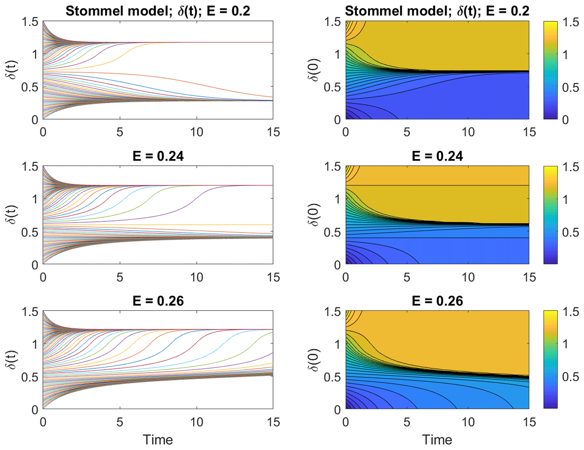
Figure 5

Finally, for E = 0.26 (bottom row), there is no thermally dominated equilibrium anymore; some of the trajectories approach the (now unique) equilibrium quickly, while those starting from a small initial value hover near the (now vanished) steady state, its influence still there. But one by one, the trajectories undergo a rapid transition to the salinity-dominated equilibrium. The transition region between orange and blue colours is not horizontal anymore, as it was for E < 0.25, indicating that sooner or later, all initial conditions lead to the salinity-dominated equilibrium.

In summary, we have seen here the explicit comparison of positive and negative feedback in (8); the visualization of stability and instability through phase-space velocity together with equilibrium curves in (12)–(14) and Figure 3; the visualization of stable and unstable equilibria through the Lyapunov potential in (16), (17), and Figure 4; and finally the emphasis on the stable equilibria through the analytical time-dependent solution in (18), (19), and Figure 5. Each perspective offers a different insight, and they thus reinforce each other.

6. Epilogue: Personal and Scientific Musings

The history of Stommel (1961) is particularly dear to me, because this paper ultimately was the one that started my own research career. And as Figure 6 shows, the great Henry Stommel took note of the work by a PhD fresh out of graduate school. I am grateful to the Tellus editors that they have allowed me to present this mix of historical and scientific aspects. The reception of Stommel (1961) shows one more time how circuitous the flow of scientific ideas can be. Despite the substantial caveat on the dynamics, Stommel’s 1961 Tellus paper now rightfully counts as one of his—and thus the field’s—most important ever.

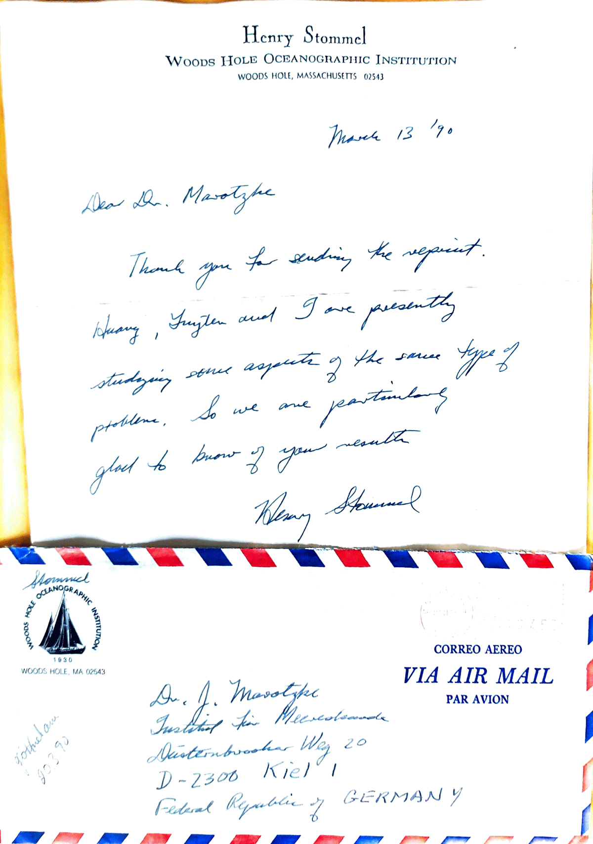
Figure 6