
1 Introduction
Many processes of interest in the Earth system, such as the movement of water or the cycling of biogeochemical elements, can be conceptualized as streams of material that pass through interconnected reservoirs. We can think of them as continuous flows of mass passing through the atmosphere, the oceans, and the biosphere, or through subsets of these reservoirs. To gain insights into overall system dynamics, it is thus natural to ask how long it takes for mass flows to pass through a system composed of multiple and potentially interconnected reservoirs. Furthermore, given the magnitude and scale of human modification of the Earth system, it is relevant to ask questions about how anthropogenic activities modify the duration or timescales at which mass flows operate in the Earth system.
Within the context of this article, the term timescale refers to the duration or time length at which natural phenomena occur, and the range that these time lengths exhibit in nature. Timescales are different than timelines, which are a series of events organized chronologically, as in the geologic time scale (words separated by a space) that represents the sequence of major events in Earth’s history. Timescales, on the contrary, are generally independent from a specific calendar and measure lengths of time at which processes occur. There are a number of metrics used in the scientific literature to characterize timescales, which include terms such as turnover time, residence time, lifetime, response time, among others, and unfortunately, there is much confusion about what each of these terms mean and how they should be calculated from data and models. Nevertheless, these timescale metrics are of fundamental importance to characterize the dynamics of natural processes.
Timescale questions are common in diverse scientific fields such as hydrology (Benettin et al., 2022; Ginn, 1999; McGuire and McDonnell, 2006; Sprenger et al., 2019), atmospheric transport and chemistry (Junge, 1974; Lindqvist and Rodhe, 1985; Prather, 1996; Waugh and Hall, 2002), biogeochemistry (Carvalhais et al., 2014; Dettmann, 2001; Friend et al., 2013; Lu et al., 2018; Manzoni et al., 2009; Rasmussen et al., 2016), ocean sciences (Delhez et al., 1999; Deleersnijder et al., 2001; Monsen et al., 2002; Takeoka, 1984), among other disciplines. For example, a prominent question that has been central in the development of concepts and methods for obtaining timescale metrics is how long would it take for the natural carbon cycle to remove from the atmosphere CO2 of fossil-fuel origin? (Bolin, 1980). To address this and many other timescale questions, it is of fundamental importance to develop an abstract conceptual theory of timescales of Earth system processes.
A number of publications in Tellus have been key for establishing the basis of a general approach to study timescale questions in Earth system science (ESS) (e.g. Bolin and Rodhe, 1973; Björkström, 1978; Lewis and Nir, 1978; Nir and Lewis, 1975; O’Neill et al., 1994; Rodhe and Björkström, 1979). This approach was developed following a very general mathematical framework to study natural systems as open dynamical systems. It was recognized that diverse systems in biology or the geosciences can be represented abstractly as systems in which some material enters through an observer-defined boundary, the material stays in the system for some period of time, it may change positions inside the system, and eventually leaves the system through the system’s boundary (Eriksson, 1961, 1971; Rodhe, 2000). Using this abstraction, it is possible to develop concepts to help answer diverse timescale questions across multiple scientific disciplines. The main recognition was that it was convenient to express scientific questions in terms of time intervals with respect to the time of entrance and exit of material to the system of interest (Figure 1). In other words, by expressing time as relative to the time of entrance of material into the system, it is possible to ask questions about the age of material present in the system, or the age of material when it exits the system.
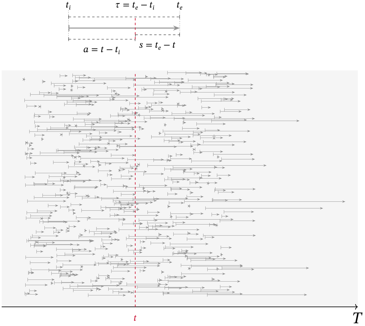
Figure 1
Timescale metrics such as age, transit time, and survival time represented as time intervals at which a stream of particles passes through an open system. T represents the reference time frame over which time events are recorded for each particle. These time events are the time of entry to the system ti, and the time of exit te. For each time of observation t, it is possible to obtain the age of particles inside the system as the interval , and their survival time as (making a prediction about their future behavior). Also, at each t it is possible to quantify the transit time for those particles leaving the system at . As t changes (e.g., sliding the red dashed line forward), the values of a, , and s change with time. At the macro scale, we are interested in the statistical behavior of the ensemble of particles (probability distributions and their moments) of the intervals a, , and s as they change with t.
The early concepts developed in Tellus articles have matured considerably and important advances have been published in the previous decades. On the occasion of the 75th anniversary of Tellus, it is my aim with this article to review part of the previous history of development of timescale concepts in ESS, and to briefly review some of the most significant advances in this field. In addition, I present some opportunities to address new questions that are now possible to study using the recent theoretical and computational developments.
This article is organized as follows. First, I review the development of timescale concepts in ESS and how the journal Tellus contributed to these developments. Then, I review some of the most important recent advances, drawing mostly from progress made in hydrology and carbon cycle science. I provide then a mathematical synthesis of the framework that allows one to ask timescale questions for nonlinear systems out of equilibrium. Given my own work on the carbon cycle, I present an example on the use of these concepts to address problems related to the emissions of fossil-fuel carbon and the time it would take to remove this extra carbon from the atmosphere–land–ocean system. At the end, I present an overview of the new type of scientific questions that the new emergent theory provides, and how scientists across ESS can take advantage of these theoretical developments.
2 Historical Development of Timescale Concepts
Erik Eriksson, former head of the Swedish Meteorological Institute and key contributor to Tellus, was perhaps the first to introduce a general conceptual framework to analyze natural reservoirs and their timescale characteristics (Eriksson and Welander, 1956; Eriksson, 1961, 1971). He conceptualized the mass stored in a reservoir, say water, sediments, carbon, gases, etc, as being composed of infinitesimal units of a given age. This age is defined as the time that the material units have since they entered the reservoir until a time of observation. Therefore, one can characterize the mass stored in a given reservoir according to a cumulative distribution function of ages, or equivalently, according to a probability density function (pdf) (Eriksson, 1961). Eriksson provided formal definitions of the terms turnover time and residence time, the latter subsequently renamed as transit time (Bolin and Rodhe, 1973; Eriksson, 1971). He also showed that there was a connection between the age of masses stored in the reservoir and the age of mass in the flux out of the reservoir. However, the concepts introduced by Eriksson were difficult to grasp, the mathematics were convoluted, and no clear formulas were given about how to compute these quantities in practice; only the theoretical concepts were presented in this early work.
Bolin and Rodhe (1973), in a short article published in Tellus, brought much more clarity to the problem, simplified the mathematics, and reaffirmed the three fundamental timescale metrics that must be distinguished among each other, namely the turnover time, the age, and the transit time. They also showed that there are three possible relations between the mean age and the mean transit time: (a) the mean transit time is higher than the mean age, indicating that material units entering the reservoir have a low probability of exiting early and remain stored in the reservoir for some time until their probability of exit increases as they become older. Björkström (1978) showed that there is a theoretical upper limit to this relation, in which the mean transit time cannot be larger than two times the value of the mean age (Figure 2). An extreme example of such a theoretical limit would be a piston-flow system in which the material enters at one end of a cylinder and it is pushed at a constant speed towards the other end until it leaves, with a mean transit time equal to two times the mean age. (b) Mean age and mean transit time are equal, which only occurs in single well-mixed compartments where each material unit present in the compartment has the same probability to appear in the output flux. The well-mixed property for single compartments is often misunderstood; it does not imply that all particles inside the compartment have the same age, it only implies that all particles inside the compartment have the same probability to appear in the output flux and therefore can leave at any age. Well-mixed compartments are characterized by a simple exponential distribution of age and transit time. (c) The mean age is higher than the mean transit time, indicating that material units entering the reservoir have a higher probability of exiting than the material units already present in the reservoir (Figure 2). This type of system seems to be more common in nature.
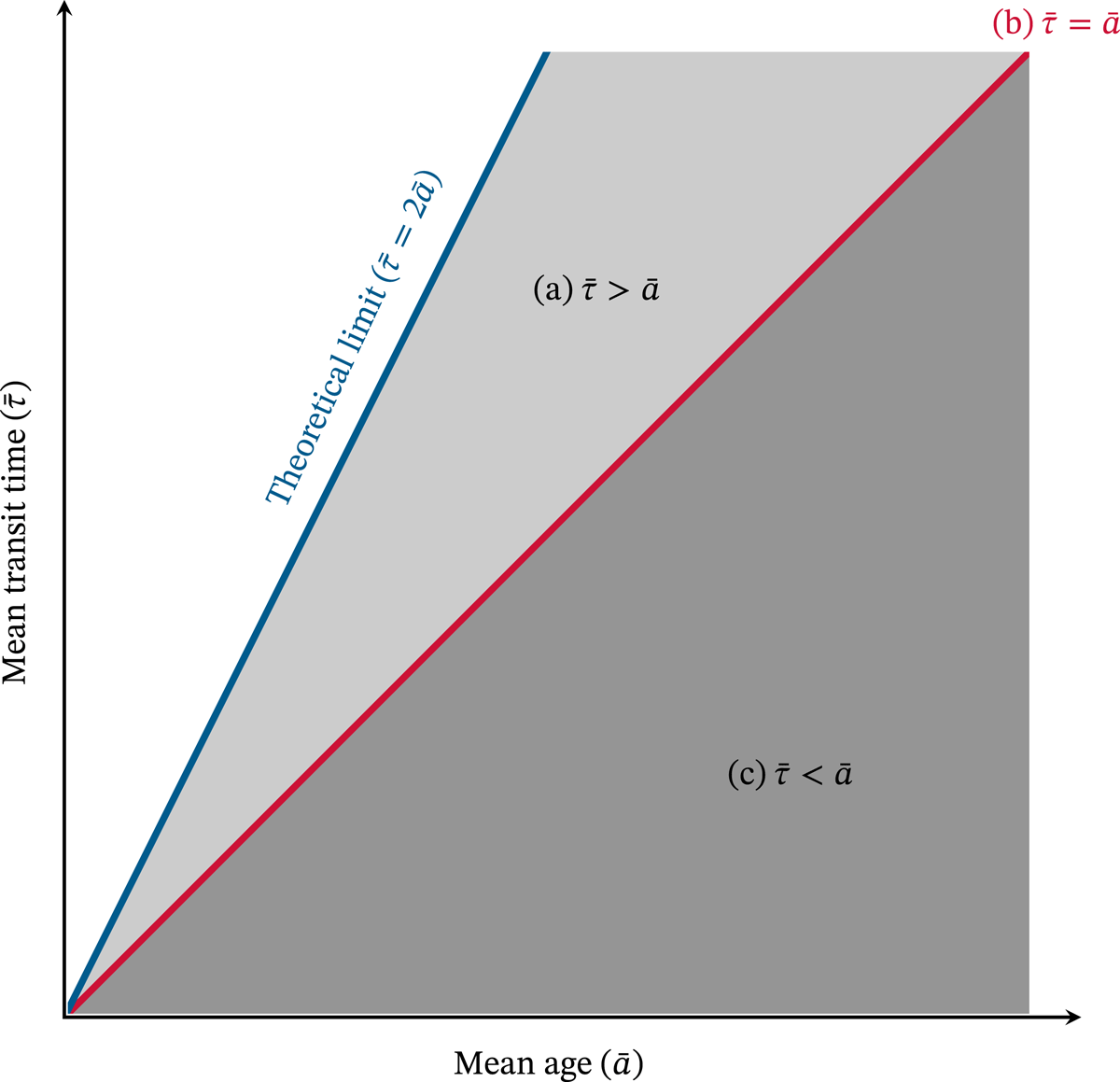
Figure 2
Space of potential relationships between mean age () and mean transit time () for systems in equilibrium (after Bolin and Rodhe, 1973; Björkström, 1978). (a) Mean transit time > mean age (light gray region), indicating that particles entering the system have a low probability of appearing early in the output flux. (b) Mean transit time = mean age (1:1 line), indicating that the system is well mixed and all particles stored have the same probability to appear in the output flux. (c) Mean transit time < mean age (dark gray region), indicating that particles entering the system have a high probability of leaving early. Region (a) has an upper theoretical limit defined by the 1:2 line, which corresponds to the case of an idealized piston-flow system in which all particles leave after completely traversing the system, thus (c.f. Björkström, 1978; Calabrese and Porporato, 2015).
These concepts were initially developed under the framework of systems in equilibrium, where the total material stored in the system does not change over time. Therefore, the distributions of age and transit time are unique time-invariant functions. While this assumption may be reasonable under some circumstances and the unique distributions may provide relevant insights about the timescales of material cycling in reservoirs, it may not be a reasonable assumption for many systems and problems of interest.
Two articles in Tellus (Lewis and Nir, 1978; Nir and Lewis, 1975) expanded the theory of timescales for non-equilibrium systems using linear response theory and convolutions of time-dependent functions. They provided a very comprehensive treatment of the non-equilibrium problem, but they did not develop methods for obtaining the response functions needed to compute time-dependent timescale metrics. Nevertheless, two important concepts emerged from these articles: (1) for systems out of equilibrium, the age distribution is a time-dependent function, which can be expressed as a pdf that changes over time (Figure 3). This implies that every time we observe the system there is a different age distribution. One can also think about this time-dependent age distribution as a three-dimensional surface where the three axes are time, age, and the proportional contribution of mass to the total mass in the system. (2) The concept of transit time must be separated into two distinct concepts, depending on whether one is looking at the transit time of current inputs, or the transit time of current outputs. These two concepts are now called the forward transit time and the backward transit time, respectively. The forward transit time represents the time that it will take current inputs to appear in the output flux, while the backward transit time represents the time that it took current outputs to pass through the system since they entered (notice the difference between future and past tense in these definitions).
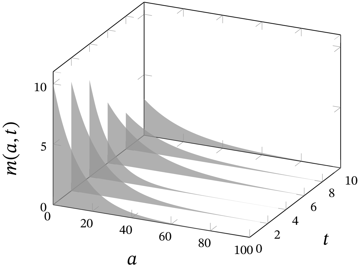
Figure 3
Probability distribution of mass stored in a system as a function of age a and time t. For simplicity of presentation, this plot shows slices of the three-dimensional distribution for discrete values of t, but in reality, the distribution is continuous in time. In this example, the distribution changes from an initial state (front) with large storage of mass of young ages, toward less total mass and of older ages. For each value of t, , i.e., the gray area under the curve is the total mass stored in the system at each t.
These articles (Lewis and Nir, 1978; Nir and Lewis, 1975) contributed to better understand the complexity of the problem for systems out of equilibrium, and how to interpret results from tracer studies in relation to these theoretical quantities. However, these authors did not provide explicit formulas for the computation of time-dependent age and transit time distributions. It would take several decades until the first approaches would emerge to be able to deal with practical computations of timescales for nonlinear and time-dependent systems. Meanwhile, a confusing misuse of formulas and concepts were applied across disciplines, with some authors using the concepts of age and transit time interchangeably, ambiguously using the term residence time to refer to turnover time, survival time, age, or transit time, using the simple formulas of the one-single-reservoir case for systems with multiple reservoirs and connections among them, and using assumptions of equilibrium for system clearly out of steady state (Benettin et al., 2022; Monsen et al., 2002; ONeill et al., 1997; Sierra et al., 2017).
3 Recent Progress for Assessing Timescales in Systems Out of Equilibrium
Watershed hydrology is one branch of ESS where important progress has been achieved in obtaining age and transit time distributions for non-equilibrium systems (Benettin et al., 2022; Botter et al., 2011; Harman, 2015; van der Velde et al., 2012). The main conceptual advance in this field has been the further development of methods based on functions that result from dividing a transit time distribution by an age distribution. These functions, which are called StorAge Selection (SAS) functions, can change over time and can be integrated to rank parcels of water in numerical simulations that effectively compute time-dependent transit time distributions (see review by Benettin et al., 2022).
Despite these important advances, the work in watershed hydrology has been limited to the analysis of the water balance of the catchment, a system with one single input flux (precipitation) and two or three output fluxes (evaporation, transpiration, runoff) without a clear definition of internal components where water may be temporarily stored. For this reason, it has been difficult to translate the results from watershed hydrology to other systems where the mathematical description of inputs, outflows, and internal compartments may be very different and more complex.
Progress toward theoretical generality appeared in the contribution by Rasmussen et al. (2016), who derived equations for mean age and mean transit times for systems out of equilibrium, the so-called non-autonomous systems. They provided explicit equations that can be applied to a very large type of dynamical systems used in the bio- and geosciences, with the only requirement that the system of ordinary differential equations describing the dynamics is mass balanced. These systems are defined as compartmental dynamical systems (Anderson, 2013; Jacquez and Simon, 1993) and they have important mathematical properties that restrict the set of behaviors that can be observed from these systems. Mathematically, a compartmental system can be written as the sum of a vector of material inputs to well-mixed compartments, and a matrix–vector product that encodes all the exits from the compartments and transfers among them. This matrix, called the compartmental matrix, can include functions that nonlinearly relate the mass of the different compartments. The compartmental matrix has three important properties: all diagonal elements are non-positive, all off-diagonal elements are non-negative, and the sum across rows for each column produces a non-positive value. Therefore, any mathematical model of differential equations describing the dynamics of mass in sets of reservoirs that exchange mass among each other and with an external environment can be expressed as a compartmental system. Time-dependent timescales can be computed for the entire system and for the individual compartments. This includes models of the carbon cycle and any other biogeochemical element, as well as models in hydrology and atmospheric sciences.
Building on the mathematical framework of compartmental systems, Metzler et al. (2018) developed methods to obtain entire age and transit time distributions for non-autonomous systems, even for those that are nonlinear. This new approach is based on a linearization procedure of the solution trajectory of a mass-balanced model, and produces distributions of age and transit time that change over time according to changes in the rates of mass transfer in the system. With this approach, it is thus possible to study timescale questions for any mass-balanced model, provided that it can be expressed mathematically as a compartmental system.
4 A General Framework for Time-Dependent Timescales
In this section, I provide formal definitions of timescale metrics synthesizing recent developments in hydrology and carbon cycle science. Readers not interested in the mathematical details can skip this section and learn about applications of the theory in the next section. The treatment of reservoir theory presented here is an extension of the concepts originally presented in Bolin and Rodhe (1973), expanded to the non-equilibrium case using the recently developed theory (Benettin et al., 2022; Botter et al., 2011; Calabrese and Porporato, 2015; Metzler et al., 2018).
4.1 General characterization of age and transit time distributions
Consider an open system, potentially containing multiple interconnected compartments, that receives and releases material through its boundaries. This material is characterized by its mass, and we will consider the total mass stored in the system, in the input flux, and in the output flux. We will also consider these masses as composed of small units that could be interpreted as individual atoms or molecules, which, for generality, I call particles from now on. In addition, I consider two different representations of time, a time dimension T that serves as a reference frame for the observer and can be expressed as a calendar time; and as time intervals between events occurring on T (Figure 1, Table 1). When particles enter the system, the event of their time of entry or injection is recorded as ti, and the time when they exit as te. Thus, the time interval is defined as the transit time of individual particles traveling through the system. Observing the system is also an event, and it occurs at t. Thus, we are interested in the time interval between the time of entry and the time of observation of a particle inside the system, , and we define this interval as the age of the particle. The interval between observing the particle in the system and its time of exit, , is defined as the survival time, which has also been called residual or remaining life expectancy (Nauman, 1969, 2008). Although the survival time has not been addressed in detail in most previous publications (however see Calabrese and Porporato, 2015), it emerges from the same conceptual basis as age and transit time. These three metrics are related by the expression (Figure 1).
Table 1
Summary of symbols and definitions.
| SYMBOL | DESCRIPTION | EXPRESSION |
|---|---|---|
| Events | ||
| t | Time of observation on a timeframe T | |
| ti | Time of entry or injection of single particles | |
| te | Time of exit or ejection of individual particles | |
| Intervals | ||
| a | Age of individual particles | |
| Transit time of individual particles | ||
| s | Survival time of individual particles | |
| Distributions | ||
| pdf of age a at time t | ||
| pdf of transit time at time t | ||
| Distribution of mass of age a at time t | ||
| Distribution of mass in flux with transit time at time t | ||
| Cumulative distribution of mass with age at t | ||
| Cumulative distribution of flux with transit time at t | ||
| Aggregated quantities | ||
| M(t) | Total mass in the system at time t | |
| F(t) | Total flux (in or out) of the system at time t | |
The theory of timescale characteristics in Earth system processes is based on the macroscopic characterization of the time intervals just defined. These intervals are treated as random variables for which probability distributions and their moments can be computed. The traditional theory for systems in equilibrium is only based on the characterization of the properties of these intervals, and it assumes that the time when particles enter is irrelevant. For systems out of equilibrium, the theory considers both the reference time frame where events occur and the intervals between events (Rasmussen et al., 2016).
In the general theory for systems out of equilibrium, we are interested in describing the timescale characteristics of the mass stored in the system at any given time M(t). Because we assume that the total mass is composed of particles that have entered the system in the past and have a certain age at the time of observation, we can express the total mass as a cumulative distribution function M(a,t) over the variable a for fixed values of t (i.e., a marginal distribution). We assume that as we accumulate mass over increasing values of age, the function has a well-defined limit
Equivalently, the total mass in the system at t can be expressed in terms of a pdf of ages as
where the prime symbol in a’ indicates the dummy variable of integration, and for all values of t. Differentiating this equation with respect to a and rearranging terms yields
Thus, the pdf of ages of mass stored in the system can be interpreted as the relative sensitivity of the cumulative mass function with respect to ages.
A similar characterization can be made for the fluxes in or out of the system with respect to the variable transit time . However, for systems out of equilibrium, it is necessary to differentiate between the transit time of particles arriving at t that will have a future transit time, versus the particles being released out of the system at time t that had a past transit time. We refer to these different forms of transit time as the backward and the forward transit time, respectively. For simplicity of exposition, we will focus for the moment on the backward transit time and assume that the flux F(t) represents the output flux from the system at time t (in section 4.4, the theory to the forward case is expanded). In analogy to mass storage, this flux can be characterized by a cumulative distribution function with an upper limit
which can also be expressed in terms of a pdf
with . This equation can be manipulated to express the transit time pdf as
Similarly, a cumulative distribution function and a pdf for the survival time can be defined as for age and transit time. However, they are not presented here due to space limitations and because they are not relevant to the theory presented below.
4.2 Relationships between age and transit time distributions
The age and the transit time pdfs are of particular interest in many scientific disciplines, and most efforts shall concentrate on obtaining estimates of these functions. For the special case of systems in equilibrium, these two functions are related in a closed mathematical form (Bolin and Rodhe, 1973; Björkström, 1978). For systems out of equilibrium, their relationship is less straightforward (however, see O’Neill et al. (1994) for a closed-form relationship between the means of these distributions), and for this reason their relation is better studied using the ratios
These are different forms of the so-called SAS functions used in watershed hydrology (Benettin et al., 2022), and they can be used to infer the proportion of the storage of mass at different ages that is selected for release in the output flux. Equation (8) in particular, can be interpreted as the probability that the mass of a certain age will be released out of the system at a particular time, or as the removal rate in units of inverse time. Using equations (3) and (6), and the fact that , we can express equation (8) as
which can be interpreted as the change in the cumulative transit time distribution at time t generated by a change in the cumulative age distribution at t.
The particular shapes of the functions of equations (7) to (9) at each value of t provide very useful information about how the output flux “selects” (as in statistical selection) mass across the range of available ages to be released out of the system. Thus, three type of shapes are possible: (a) most of the mass that appears in the output flux is composed of old age, (b) the mass in the output flux is uniformly selected across the entire range of available ages of stored mass, and (c) the mass in the output flux is preferentially selected from young ages of mass stored (Figure 4). These three cases generalize the three cases for the means described by Bolin and Rodhe (1973) for systems in equilibrium (Figure 2), and offer a powerful approach to study overall characteristics of system dynamics.
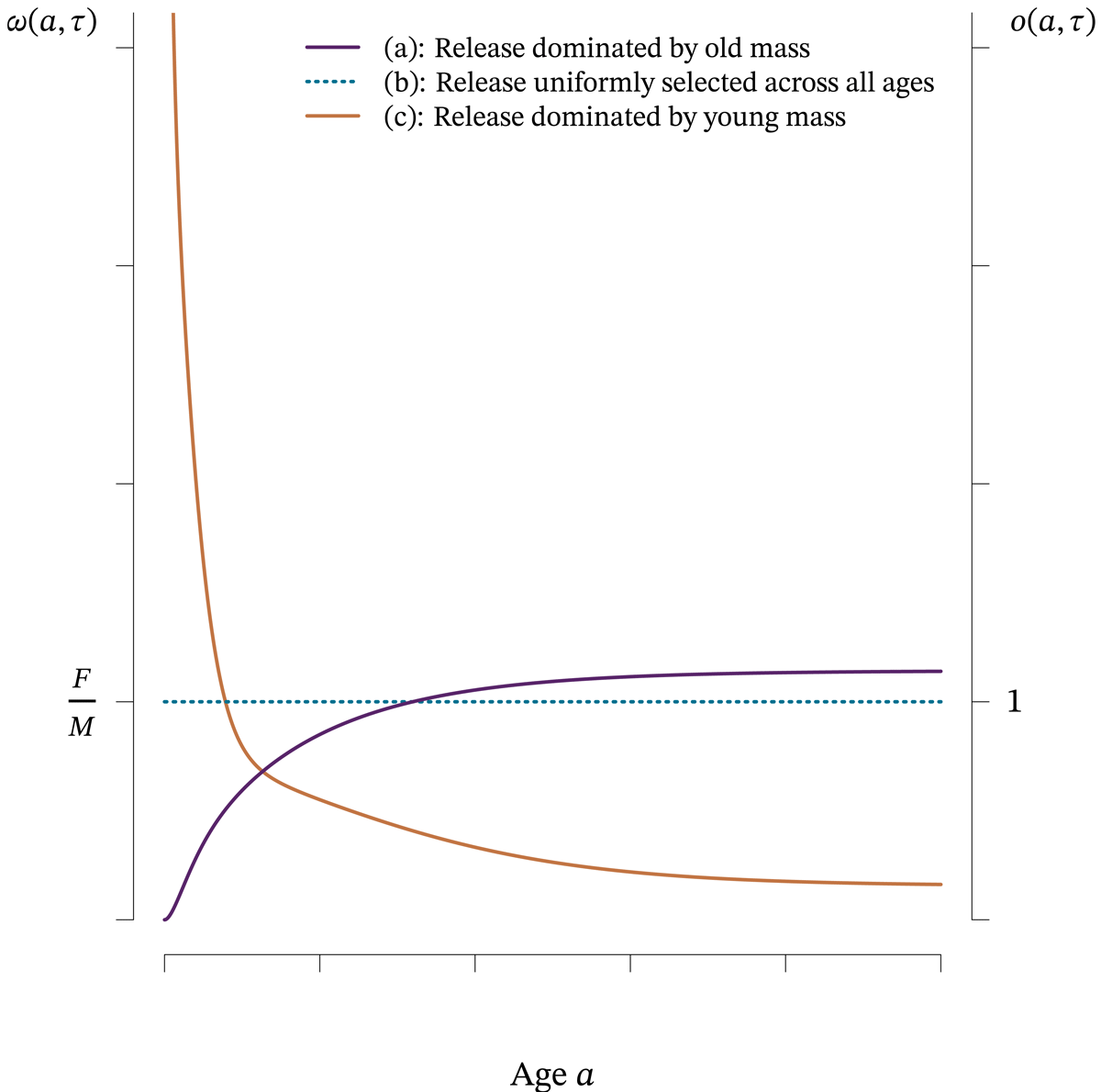
Figure 4
Possible shapes of the functions and for fixed values of t. The shape of these functions represents three potential cases: (a) the release flux is dominated by old mass, (b) the release flux has similar ages as the mass stored, and (c) the release flux is dominated by young mass. These three cases generalize the simple cases for mean values at equilibrium defined by Bolin and Rodhe (1973) (Figure 2). Notice that is a scaled version of (equations 7 and 8); therefore, in case (b) the values of converge to the ratio F/M.
4.3 General solution of the time-dependent age distribution
So far, nothing has been said about how to obtain the different forms of age and transit time distributions. Working independently, researchers in hydrology (Botter et al., 2011; Harman, 2015; van der Velde et al., 2012) and in carbon cycle (Metzler et al., 2018; Rasmussen et al., 2016) have developed methods to obtain age and transit time distributions for systems out of equilibrium. The approach in hydrology uses time-series observations of precipitation and run-off and makes no assumptions on the internal structure of the system. The approach parameterizes forms of the SAS functions to obtain solutions of transit time pdfs that match the observed data. In contrast, the approach in carbon cycle science relies on an available model expressed as compartmental dynamical system that makes explicit assumptions about the structure of the system as a set of compartments that exchange mass among each other, potentially including nonlinear functions that determine rates of mass exchange and release.
Despite differences in these two approaches, the new methods to obtain time-dependent age and transit time distributions have one important aspect in common, and it is the representation of the problem in the form of the McKendrick–von Foester equation (Keyfitz and Keyfitz, 1997). In mathematical biology and demography, the McKendrick–von Foester equation generalizes problems in which the size of a population (number of individuals, expressed as a function of age and time ) changes with respect to a and t simultaneously as
where is the rate of removal (mortality in population studies) with respect to age a at time t. This equation expresses the fact that the rate of change of the population with respect to time at age a exactly balances the rate of change with respect to age after accounting for the rate of removals.
For mass balance problems, the McKendrick–von Foester equation can be expressed as
where we interpret as the rate at which mass is selected from the total mass across the range of ages. To obtain a particular solution for this equation, it is necessary to include an initial distribution as initial condition
representing the distribution of ages of the population at ; and the boundary condition
expressing the fact that all flux inputs (newborns in population studies) have, by definition, an age of zero.
There are a number of mathematical methods available to solve equation (11) (Keyfitz and Keyfitz, 1997), which yield an analytical or numerical expression for . Nevertheless, an expression for must be provided, which for a compartmental dynamical system is straightforward to specify because it emerges from the mass balance equations out of the compartments; i.e., the term emerges directly from the compartmental matrix (Metzler et al., 2018; Rasmussen et al., 2016). When a model is not available, as in the case of watershed hydrology problems, the proposed approach is to use an empirically parameterized SAS function to specify how the output flux selects from the available ages in storage (Benettin et al., 2022). Readers interested in the application of these methods can obtain additional details and access to software in Metzler et al. (2018), Benettin and Bertuzzo (2018), and Harman and Xu Fei (2024).
4.4 Forward and backward transit times
Once a solution for is obtained, and given that M(t) is known, it is then possible to calculate the time-dependent age pdf and the time-dependent cumulative distribution using the equations presented above. To obtain the time-dependent forward and backward transit time distributions, we take advantage of the complete knowledge of the time evolution of the distribution of ages, and the fact that time-dependent input and output (exit) fluxes are also known.
We now define the backward transit time distribution function as a (exit) flux-weighted pdf of transit times. From equation (8), it can be obtained as
Similarly, we define the forward transit time distribution function as a (input) flux-weighted pdf of transit times
which implies that we have knowledge of the future dynamics of the inputs up to an arbitrary long time .
Notice that for a fixed value of t in a non-equilibrium system, . This is because input and output fluxes are not necessarily the same for a given t, and the functions and m change over t. Conversely, for systems in equilibrium where , and and m are unique, it is well known that (Niemi, 1977). In addition, if we focus on the behavior of one single particle injected at a fixed time ti and exiting at a fixed time te, we obtain the equality (Metzler et al., 2018)
In words, the transit time for an individual particle is the same independently if one looks at the time it enters or at the time it leaves the system. This equality not only applies to one single particle, but also to the set of particles that simultaneously arrive at ti and exit together at te, which could be a very small subset from all particles in the input and output fluxes. However, this behavior for one individual particle or a small subset of particles does not scale up for the total fluxes because all particles entering at one single time leave at different future times, and the flux of all particles exiting at one single time entered at different past times.
In addition to these transit time distributions, it is also possible to obtain time-dependent survival time distributions . They provide additional insights about the future behavior of mass stored in a system. The survival time distributions are at the same level of importance as age and transit time distributions and complement the information provided by them (Figure 1). These three distributions are mathematically related and therefore connected via the SAS functions. Thus, one can obtain survival time distributions from knowledge of the other complementary distributions (Calabrese and Porporato, 2015).
5 Application of the Theory to Problems in ESS
5.1 The transit time of anthropogenic CO2
The question of how long would it take to remove from the atmosphere CO2 of fossil-fuel origin? has been a main source of motivation for the development of a theory of timescales of material cycling in natural systems, particularly for the early founding figures of Tellus. For instance, Rodhe (1991, p. 4) in his memoir on Bert Bolin, writes “After Bert Bolin finished his Ph.D. in 1956, C.-G. Rossby advised him to move into another research area: atmospheric chemistry and questions specifically related to the residence time of pollutants in the atmosphere. That is when his interest in the carbon cycle started.” Therefore, I think it is fair to assert that most of the early theoretical development on the topic of timescales were motivated by the question of the timescale characteristics of anthropogenic CO2. However, this has been proven to be a difficult problem.
Carbon in fossil fuels has been isolated from other components of the Earth system for very long times. Once this carbon is burned by humans, it enters the active part of the global carbon cycle. It enters the atmosphere as CO2 where it remains stored for some time, and eventually, this carbon is transferred to the terrestrial biosphere, or to the oceans where it would remain stored for some period of time. This anthropogenic carbon can return to the atmosphere, either by the respiratory activity of organisms on land and oceans, or by inorganic ocean-atmosphere exchange. Therefore, the question of how long anthropogenic carbon remains in the atmosphere could be studied from two different points of view. From the point of view of the isolated atmospheric compartment and only considering the initial transfer, from burning of fossil fuels until CO2 uptake by land or oceans; or from the point of view of a larger interconnected system including the atmosphere, land, and oceans, with a final receiver geological reservoir (Archer and Brovkin, 2008; Archer et al., 2009). Because one can study this problem from these two particular points of view, a lot of confusion and debates have existed regarding this question (Gaffin et al., 1995; O’Neill et al., 1994; Tans, 1997).
In addition to these difficulties about how to define the boundaries of the system of interest, there are additional difficulties related to the nonlinearity of carbon exchange between the atmosphere with oceans and land, as well as issues of time-dependencies of other external forcing factors. For these reasons, the problem of the time to remove carbon of fossil-fuel origin must be addressed under a broader conceptual framework, one that can deal with a general characterization of carbon compartments, and that can address explicitly nonlinearities and time-dependencies.
A reasonable approach to address this problem is to define an open compartmental system that has as its main input flux carbon of geological origin entering the atmosphere, and an output flux of carbon returning to a geological reservoir such as ocean sediments. Carbon is transferred among the main active compartments of atmosphere, land, and oceans, with equations defining the main transfer fluxes including potential feedback among reservoirs that lead to systems of nonlinear differential equations (Rodhe and Björkström, 1979). Rates of carbon transfer among reservoirs could also be affected by changes in climate, such as the rates of photosynthesis and respiration on land and oceans, or the rates of CO2 exchange between the atmosphere and the ocean (Kaufhold et al., 2025). Many of these processes are already represented in Earth system models (ESMs) of different levels of complexity, from reduced complexity models and simple emulators to high-resolution ESMs. Many of these models are currently under active development, improving their representation of multiple processes with their nonlinearities and feedback. More importantly, most of these models can be translated to a mathematical representation according to the formalism of nonlinear non-autonomous compartmental system (Metzler et al., 2020; Sierra et al., 2018). Then, the question of how long would it take to remove carbon from fossil fuel origin from the active carbon cycle can be addressed as a problem of finding the forward or backward transit time of a nonlinear non-autonomous compartmental system (Metzler et al., 2018), linking inputs from the burning of fossil fuels to outputs to geological storage.
Under this theoretical framework, it would be possible to learn about differences in forward transit times between anthropogenic carbon emitted in the past, versus emissions in the future under different scenarios. It would be possible to learn about ages and transit times of individual compartments, or to obtain the survival time of the current burden of anthropogenic CO2. It would also be possible to compute atmospheric warming effects attributed to emissions occurring at different times, expanding the current conceptual framework of static global warming potentials (Joos et al., 2013; Lashof and Ahuja, 1990; Rodhe, 1990). It would also be possible to learn how human activities perturb the global carbon cycle across a wide range of timescales and how these perturbations are exacerbated over time as emissions continue, or mitigated as emission policies are implemented. This type of analysis could be readily implemented using simple models such as FaIR (Leach et al., 2021) or BernSCM (Strassmann and Joos, 2018) combined with existing tools for timescales analysis, such as those developed in hydrology (Harman and Xu Fei, 2024) or for compartmental systems of the carbon cycle (Metzler et al., 2018). Overall, the implementation of such a computational framework would enable a set of new scientific questions and policy analyses.
5.2 Timescales of anthropogenic perturbations to Earth system processes
The previous example demonstrates that a general mathematical framework is essential to address a complex problem that requires a careful definition of system boundaries, a specification of nonlinearities in material exchange among reservoirs, and a clear specification of time-dependencies in forcing that alter rates of material exchange. It also shows that for such complex problems, one must also be specific about the type of questions being asked. Because the forward and backward transit times are different for systems out of equilibrium, one must be careful in either posing questions on the future dynamics of current material inputs or the past dynamics of current outputs. Given the extent and magnitude of human modification of material cycles in the Earth system, it is reasonable to expect that the age and transit time distributions for many material cycles have been drastically modified over the past one-and-a-half century. Therefore, scientific questions about the timescales of material cycles should move from attempts to identify single values of a timescale metric to new questions about the magnitude and direction of their perturbation.
Two areas with potential for new scientific developments regarding the application of timescale metrics are: the timescales of reactive nitrogen in the environment, and the modification of the timescales of methane in the atmosphere. Although there are many other areas with large potential for applications, I present here these two as clear examples where progress can be achieved within the next years.
Although the atmosphere stores large amounts of nitrogen (N), this N is not easily available for organisms on land and oceans because it is present as inert N2 gas, with a triple covalent bond between the two N atoms that is very difficult to break. Since the beginning of the industrial revolution, humans have increasingly added reactive nitrogen to the environment by burning fossil fuels, by promoting the cultivation of species that can fix N, and by artificially producing reactive N through the Haber-Bosch process to produce fertilizers (Galloway et al., 2021). This reactive nitrogen is cycled among terrestrial ecosystems, the atmosphere, and aquatic ecosystems, in a chain of biogeochemical reactions collectively known as the nitrogen cascade (Fowler et al., 2013; Galloway et al., 2003). During the time reactive N stays in these reservoirs, it produces a number of negative environmental impacts, which include: contribution to the greenhouse effect by N2O, increases in the production of tropospheric ozone that acts as air pollutant, acidification of precipitation, eutrophication of aquatic ecosystems, and changes in the biodiversity of terrestrial and aquatic ecosystems, among other impacts (Galloway et al., 2003). Eventually, reactive nitrogen is denitrified and returns to the atmosphere as N2.
The time that anthropogenic reactive nitrogen spends in the natural environment is currently unknown. Although there are broad estimates of the timescales of reactive N in individual reservoirs, such as atmospheric N2O (Prather et al., 2015) or in global soils and oceans (Fowler et al., 2013), there are no estimates linking these different reservoirs through the pathways in which reactive N moves across the Earth system. It is likely that through nonlinear interactions with the carbon and the phosphorous cycle (Gruber and Galloway, 2008), the forward transit time of reactive nitrogen will increase, spending more time in different reservoirs and exacerbating a number of environmental problems. As more reactive nitrogen is available for net primary production, more nitrogen is stored in organic compounds and could be cycled between ecosystems and food production systems, increasing its overall transit time. I believe there is an urgent need to address this problem so better policies for environmental management of N can be developed, taking advantage of the new theoretical and computational developments in the calculation of transit times, integrating new datasets and models of the global nitrogen cycle.
Another important anthropogenic perturbation is the growth rate of methane (CH4) in the atmosphere and its “lifetime.” As opposed to CO2, the trend of atmospheric CH4 mole fraction has not increased steadily with emissions, but it has shown periods of rapid growth and periods of relatively constant values (Dlugokencky et al., 2011; Saunois et al., 2025; Turner et al., 2019). Although there are large uncertainties regarding the rate of increase of different emission sources, there seems to be good agreement that the main sink of CH4, its oxidation with OH, has changed over time (Folberth et al., 2025; Lelieveld et al., 1998; Stevenson et al., 2020; Turner et al., 2019). The availability of OH has a strong influence on the so-called lifetime of methane, with a number of studies showing that as OH increases in the atmosphere, the reaction rate with CH4 speeds up and therefore CH4 spends less time in the atmosphere. However, the chemistry of CH4 in the troposphere is relatively complex, with multiple interactions with other gases such as O3, CO, NOX, among others, which have a nonlinear influence on different reaction rates and therefore affect CH4 lifetime (Lelieveld et al., 1998; Prather, 2007). This lifetime of CH4 has been quantified as the ratio of the total atmospheric mass to the total sink flux, which is equivalent to the turnover time. It is well-established that this estimate of turnover time is not equivalent to the concepts of age or transit time for nonlinear non-equilibrium systems (Bolin and Rodhe, 1973; Lewis and Nir, 1978; Metzler et al., 2018; Rasmussen et al., 2016; Sierra et al., 2017), and therefore most of the literature on CH4 lifetime has been performed with methods that do not correctly inform about the time that CH4 molecules spend in an atmosphere out of equilibrium. This is problematic because CH4, as one of the major greenhouse gases, is very relevant for the development of policies for climate change mitigation. In the policy arena, the concepts of global warming potentials and carbon dioxide equivalents are used extensively to design climate change mitigation actions, and these concepts rely on estimates of CH4 lifetime for their computations. Therefore, it is very important to improve estimates of CH4 lifetime, ideally as a CH4 transit time or survival time distribution that changes over time, using the appropriate set of concepts and formulas for nonlinear non-equilibrium systems.
Fortunately, estimates of CH4 transit time can be readily obtained using the recent set of methods discussed here applied to conceptual models (Prather, 1996, 2007) or simulation output (Stevenson et al., 2020). For instance, Prather (2007) used a simple nonlinear model with the set of chemical reactions linking CH4 with CO and OH, studying the eigenvector and eigenvalue decomposition of the linearized system of equations at equilibrium. This simple model, or other more complex versions, can be used to analyze steady-state transit time distributions of CH4 for pre-industrial conditions using the methods developed by Metzler and Sierra (2018), and performing perturbation analyses to explore how the perturbation of other chemical species such as CO or OH change the equilibrium transit times of CH4. Furthermore, results from large-scale model inter-comparison projects (e.g. Stevenson et al., 2020) can be used to obtain time-dependent (backward) transit time distributions of CH4. This can be done by translating the methods from hydrology that rely on time series of inputs (CH4 emission sources) and outputs (CH4 sinks) to obtain parameterized SAS functions and the corresponding estimates of transit times (Harman, 2015; Harman and Xu Fei, 2024). Alternatively, one can reconstruct a compartmental model from the numerical output of the models (Metzler et al., 2020) and subsequently obtain backward transit times using methods for non-autonomous compartmental systems (Metzler et al., 2018; Rasmussen et al., 2016).
6 Summary and Conclusions
After more than five decades of research, a mature theory on timescales of Earth system process has now emerged that can be used to address a wide range of problems in ESS, particularly the timescales of anthropogenic perturbation to material cycles. This theory deals with problems in which the duration of mass flows across interconnected reservoirs or compartments is of interest, and for which flow rates may interact nonlinearly among compartments and flows may be driven by time-dependent signals.
This theory is also useful to disambiguate a number of scientific terms that have been used sometimes informally in different disciplines. In particular, it is possible now to identify three basic timescale metrics that can be used to characterize any mass-balanced system: transit time, age, and survival time. They can be characterized by probability distribution functions (densities, mass, or cumulative functions) and therefore statistics such as the mean (and other higher order moments) and quantiles can be obtained from these distributions. When a system is in equilibrium, these distributions are unique, and when the system is out of equilibrium, the distribution functions change over time.
A widely used metric is the turnover time, defined as the ratio of total mass inside the system to the total input or output flux at any given time. However, the turnover time is fundamentally different than transit time, age, and survival time by the fact that it is not defined by an intrinsic probability function, and in most cases it cannot be interpreted as a time interval of the dynamics of particles in reservoirs. However, for systems in equilibrium, the turnover time is equal to the mean of the transit time distribution. Furthermore, for a one-single well-mixed compartment system in equilibrium, the distributions of transit time, age, and survival time are all equal, and therefore the turnover time is equal to the mean of these distributions. This important fact for one-single reservoir system is a special case that could be helpful under circumstances where information is limited and the assumption of equilibrium is justified, but it also has contributed a large share of confusion in the use of formulas and interpretation of concepts related to timescale metrics.
For systems out of equilibrium, the distribution functions of transit time, age, and survival time change over time. There are now computational methods available for obtaining these distributions, which can be applied to time-series data of input and output fluxes, or to mass-balanced models expressed as compartmental dynamical systems. It took several decades for the scientific community to arrive at methods for obtaining these time-dependent distributions, and the key step was to express the problem in the form of the McKendrick–von Foester equation used in population studies. For systems out of equilibrium, transit times need to be studied from the perspective of the transit time of current inputs as the forward transit time, or from the perspective of current outputs as the backward transit time.
Other terms used in the scientific literature such as residence time, adjustment time, recovery time, lifetime, e-folding time, among others, tend to be ambiguously defined or very specific for a particular set of assumptions in models. Although they can be very useful for certain situations, it would be helpful if future studies clearly define them for the particular application and differentiate them with respect to the terms transit time, age, and survival time defined here.
The emergent theory of timescales of Earth system processes and the methods for obtaining time-dependent timescale metrics open up new possibilities to address questions on the anthropogenic modification of mass flows in the Earth system. The transit times of anthropogenic CO2, CH4, and of reactive nitrogen are important environmental problems that can be formally studied with the new methods. New studies would help to understand how human activities modify the transit times of these molecules and how they modify other temporal aspects of the functioning of the Earth system. There are likely many other important scientific questions that can be addressed with this emerging theory.