
1 Introduction
Since the pioneering work of Keeling (1960), published in Tellus, it has been well established that the concentration of atmospheric CO2 has been increasing rapidly since the start of the Industrial Revolution, which has in turn led to a rise in global average temperatures. The growth of CO2 is due to human activity, primarily the burning of fossil fuels, but with a significant contribution also from deforestation and other land-use change. As global populations, economies, and industries have expanded, their increasing energy and material demands have resulted in anthropogenic CO2 emissions that increased almost exponentially over the past 200 years. However, the atmospheric CO2 concentration has only increased by less than half of the anthropogenic emissions (Friedlingstein et al., 2024). This discrepancy is the result of significant natural carbon sinks on the land and in the ocean (Bolin, 1977; Bolin et al., 1989; Revelle and Suess, 1957).
However, land and ocean carbon sinks are not static. Terrestrial and marine carbon uptake varies over seasonal to millennial time-scales, and the magnitude of these variations depends on the responses of physical and biological processes to changes in both atmospheric composition and physical climate. These responses can either slow or accelerate the rate of climate change, leading to ‘climate-carbon cycle feedbacks’ which are a key source of uncertainty in future projections (Friedlingstein et al., 2014). The role of climate-carbon cycle feedbacks is also very evident in past climate variations. Most notably, during glacial–interglacial periods, changes in CO2 drive a significant part of the glacial–interglacial changes in temperature (Petit et al., 1999; Sigman and Boyle, 2000).
The gross uptake of carbon by land and ocean depends on the concentration of CO2 in the atmosphere. Terrestrial ecosystems sequester CO2 through photosynthesis, which is stimulated by increased atmospheric CO2 if nutrients are also available (Walker et al., 2021). Similarly, diffusion of CO2 from the atmosphere into the surface layer of the ocean is controlled by the difference in partial pressures (pCO2) between the ocean and atmosphere. As a result, since the start of the industrial revolution, land and ocean sinks have kept pace with the near-exponential increase in anthropogenic emissions, evidenced by the long-term stability of the airborne fraction of CO2 emissions (Friedlingstein et al., 2024; Jones and Friedlingstein, 2020). However, the fraction of anthropogenic emissions removed by land and ocean carbon sinks is projected to decrease under climate change (Canadell et al., 2021).
On the land, CO2 fertilisation relies heavily on sufficient nutrient supply, which, despite large anthropogenic production of reactive nitrogen (Zhu et al., 2025), is not always available (LeBauer and Treseder, 2008). Nutrient cycles in some areas remain relatively closed. Old-growth tropical forests, for example, are typically limited by phosphorus (Walker and Syers, 1976), which restricts their potential CO2 uptake in the future. Changes in climate may also take plants outside their natural ranges. In the ocean, rising sea surface temperatures and increasing dissolved inorganic carbon (DIC) concentrations reduce the rate of CO2 uptake (Egleston et al., 2010; Revelle and Suess, 1957). These effects contribute to ‘sink saturation’ and declining sink efficiency under increasing CO2, which may reduce carbon uptake and accelerate global climate change in the future (Canadell et al., 2021).
Nevertheless, it was not until the early years of this millennium that general circulation models (GCMs) of the climate began to include interactions between the climate and carbon cycle (Cox et al., 2000; Friedlingstein et al., 2001). Indeed, Tellus published an intercomparison of the first two climate-carbon cycle GCMs in 2003 (Friedlingstein et al., 2003). These models were the forerunners of what are now called ‘Earth System Models (ESMs)’, and ultimately led to the ‘Coupled Climate-Carbon Cycle Model Intercomparison Project (C4MIP)’ (Arora et al., 2013, 2020; Friedlingstein et al., 2006). C4MIP compares results from multiple ESMs using a quasi-equilibrium linear formulation that was first proposed in that 2003 paper in Tellus. This ‘’ formulation has the advantage of being very simple to use, but is unable to capture vital aspects of sink saturation.
This paper for the Tellus 75th Anniversary issue aims to summarise work on coupled-climate carbon cycle modelling (Section 2), and also to propose a long-overdue update to the ‘’ characterisation of carbon cycle sensitivities to CO2 and climate, to capture sink saturation effects (Section 3).
2 The Evolution of Coupled Climate-Carbon Cycle Models
As described above, the importance of climate-carbon interactions had been revealed throughout the last 30 years of the 20th century. Although ‘full-form’ GCMs were beginning to include coupling between the climate and the ocean carbon cycle on long timescales (Sarmiento and Toggweiler, 1984), these had not yet included the land carbon cycle. GCM land surface schemes, which had traditionally focused on calculating land-atmosphere fluxes of energy, water, and momentum, were diversifying to also calculate plant photosynthesis (Cox et al., 1999; Sellers et al., 1996a). Initially, this was to improve the simulation of water fluxes over land, which is heavily influenced by stomatal pores on plant leaves (Sellers et al., 1997), by making use of empirical relationships between photosynthesis and stomatal conductance (Ball et al., 1987). These second-generation land surface models therefore coupled the water and carbon fluxes, but still required prescribed fixed maps of vegetation types and land-surface parameters (Pitman, 2003; Sellers et al., 1996b).
In parallel, a separate group of researchers had begun to develop dynamic global vegetation models (DGVMs), with the aim of simulating the changing geographical distribution of vegetation types under climate change (Cramer et al., 2001). These models were derived from biogeographical models developed for palaeoclimate reconstructions (Haxeltine and Prentice, 1996; Prentice et al., 1992), but were also increasingly based on the principles of carbon and water balance (Woodward, 1987). Before the end of the 20th century, a first attempt was made to asynchronously couple a DGVM to a GCM climate model (Betts et al., 1997). However, the pieces were now in place for a GCM of the fully coupled climate-carbon system, which are today referred to as ‘ESMs’ (Randall et al., 2019).
At the beginning of the 21st century, the first ESMs were published. A group based at the UK Met Office-Hadley Centre developed a variant of the HadCM3 climate model which included representations of the ocean carbon cycle (Palmer and Totterdell, 2001) and land carbon cycle (Cox et al., 1999), and also a simple representation of vegetation dynamics (Cox, 2001). A fully coupled climate-carbon cycle run was compared to a model run with prescribed CO2 concentrations, to isolate the impact of climate-carbon feedbacks on the rate of CO2 increase and global warming. Alarmingly, this study reported that climate-carbon cycle feedbacks increased projected atmospheric CO2 by 270 ppmv, and global warming from 4C to 5.5C, by the end of the 21st century (Cox et al., 2000). The acceleration of climate change in this model was primarily due to the suppression of the global land carbon sink by climate change, which ultimately transitioned to a carbon source from about 2050 onwards, due to increased rates of soil respiration and Amazon forest dieback under global warming (Cox et al., 2004).
Independently, a group at the IPSL in France was also developing a climate-carbon cycle model (Friedlingstein et al., 2001), making use of the IPSL-OGCM1 ocean carbon cycle model (Le Quéré et al., 2000) and the SLAVE terrestrial carbon cycle model (Friedlingstein et al., 1995). Under a prescribed 1% per year increase in atmospheric CO2, this model also simulated a suppression of the land carbon sink by climate change, with land carbon uptake at the time of doubling CO2 reduced by about a quarter. These first two ESM simulations (Cox et al., 2000; Friedlingstein et al., 2001) suggested that climate change would suppress natural carbon sinks and therefore provide an amplifying positive feedback on climate change. However, the magnitude of the positive feedback differed markedly in the two models. In order to isolate the reasons for this, a collaborative study was undertaken between the French and UK groups. The resulting paper, published in Tellus (Friedlingstein et al., 2003), identified a stronger negative response of the land carbon cycle to climate change in the UK model as the key reason for the differences between them.
Prompted by these initial studies which suggested that carbon cycle feedbacks on future climate could be large but were uncertain, the C4MIP was set up to enable a cleaner comparison between the results from the growing number of coupled climate-carbon cycle models. The first phase of C4MIP used a common emissions scenario (SRES A2) and required global atmospheric CO2 concentration to be simulated internally within each model. All models produced a positive climate-carbon feedback on climate change, but with a range that differed by an order of magnitude from an extra 20 to 200 ppmv of CO2 by 2100 (Friedlingstein et al., 2006). Two further phases of C4MIP have since been carried-out, based, respectively, on the CMIP5 and CMIP6 generations of ESMs (Arora et al., 2013, 2020). These latter C4MIP studies used a simpler experimental design in which the atmospheric CO2 concentration is prescribed to increase at 1% per year, and model runs are carried out with (‘COU’; coupled runs) and without (‘BGC’; biogeochemical runs) climate effects on the carbon cycle, to separate the direct-CO2 effects (see Figure 1; Jones et al. (2016)). Each generation of C4MIP models has seen further developments. For example, additional nutrient limitations on land and ocean carbon sinks were implemented for CMIP6, and the range of carbon cycle projections has generally been reduced (Canadell et al., 2021). However, significant uncertainty remains, especially in the response of the land carbon cycle, which is also impacted by land-use change (Arora et al., 2020). As a result, methods to separate impacts on the carbon cycle remain important.
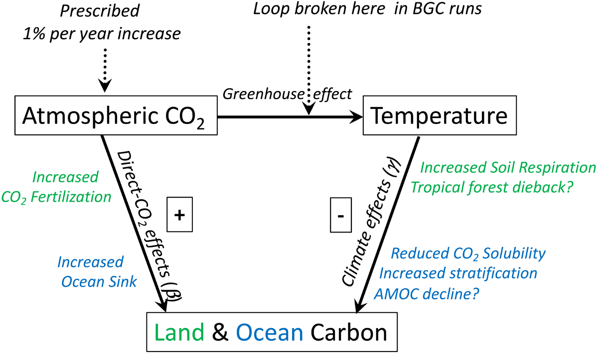
Figure 1
Schematic diagram showing the key interactions quantified in C4MIP climate-carbon cycle runs. In the latest versions of C4MIP, CO2 is not an internal model variable but is instead prescribed to increase by 1% per year. In the coupled runs, CO2 affects land and ocean carbon storage both directly (‘-effects’), and indirectly, as a result of the climate change caused by the CO2 increase (‘-effects’). In the BGC runs, the climate change effects are disabled by breaking the link between CO2 and climate. In this study, climate effects are defined as the difference between the BGC and coupled runs.
2.1 Standard – diagnosis of carbon cycle sensitivities
To quantify carbon cycle sensitivities within climate-carbon cycle models (ESMs), a standard framework has been followed since first introduced in Friedlingstein et al. (2003). Carbon cycle sensitivities are defined using two parameters: known as the carbon-concentration sensitivity (), quantifying the sensitivity of land and ocean carbon to changes in CO2, and the carbon-climate sensitivity (), quantifying the sensitivity to subsequent climate changes.
Following Friedlingstein et al. (2003), the change in global land and ocean carbon storage is assumed to be linear with increases in CO2 and also with global warming. Therefore, the future changes in land carbon storage () and ocean carbon storage () are linearly approximated as the sum of contributions from increased CO2 concentrations () and global warming (), as shown by Equations 1 (land) and 2 (ocean):
where the sensitivity parameters for land and ocean are given by , and , , respectively. Since CMIP5, the C4MIP 1% CO2 simulations have been used as the standard method for calculating these parameters. To define the parameters, the sensitivity of carbon storage to CO2 is calculated at a specific CO2 concentration (i.e., 2×CO2 or 4×CO2) using the BGC runs (isolating the direct CO2 sensitivities). The parameters are estimated using the sensitivity of carbon storage to subsequent global warming, calculated using the residual climate changes in the fully coupled simulations relative to the BGC runs (RES = COU – BGC). The and parameters for the CMIP6 ESMs are presented in Table 1, taken from Arora et al. (2020). This method of separating direct-CO2 () effects and climate () effects is demonstrated schematically in Figure 1.
Table 1
Parameters for the old formulation: land and ocean carbon-concentration ( PgC ppm-1) and carbon-climate (, PgC ) sensitivity parameters, shown for 2×CO2 and 4×CO2 in CMIP6 ESMs. As presented in Arora et al. (2020), but with values shown to just one decimal place. ∗The parameters for CNRM-ESM2-1 were recalibrated for this study.
| EARTH SYSTEM MODEL | 2×CO2 | 4×CO2 | ||||||
|---|---|---|---|---|---|---|---|---|
| ACCESS-ESM1.5 | 0.75 | –12.0 | 1.06 | –11.7 | 0.37 | –21.1 | 0.90 | –23.8 |
| BCC-CSM2-MR | 2.22 | –132.8 | 1.09 | –12.4 | 1.81 | –163.1 | 0.92 | –19.9 |
| CESM2 | 0.98 | –12.8 | 0.84 | –4.24 | 0.90 | –21.6 | 0.71 | –10.9 |
| CNRM-ESM2-1∗ | 1.36 | –48.4 | 0.62 | –4.0 | 1.36 | –83.7 | 0.57 | –9.5 |
| CanESM5 | 1.42 | –6.22 | 0.90 | –7.71 | 1.28 | 16.0 | 0.77 | –14.7 |
| GFDL-ESM4 | 1.08 | –50.7 | 0.97 | –8.97 | 0.93 | –80.1 | 0.84 | –21.7 |
| IPSL-CM6A-LR | 1.11 | –12.2 | 0.87 | –7.37 | 0.62 | –8.7 | 0.76 | –13.0 |
| MIROC-ES2L | 1.45 | –63.4 | 0.85 | –10.4 | 1.12 | –69.6 | 0.73 | –22.3 |
| MPI-ESM1.2-LR | 1.08 | –0.81 | 0.88 | –11.4 | 0.71 | –5.17 | 0.77 | –20.1 |
| NorESM2-LM | 0.94 | –15.6 | 0.88 | –9.34 | 0.85 | –21.0 | 0.78 | –19.6 |
| UKESM1-0-LL | 1.00 | –24.0 | 0.88 | –7.35 | 0.75 | –38.4 | 0.75 | –14.1 |
| Ensemble mean | 1.22 | –34.1 | 0.91 | –8.59 | 0.97 | –45.1 | 0.78 | –17.2 |
| Ensemble SD | 0.40 | 38.4 | 0.09 | 2.90 | 0.40 | 50.6 | 0.07 | 5.0 |
The quantification of land and ocean carbon cycle sensitivities in this way has been useful to identify the zeroth-order reasons for differences between ESM projections and provides a useful comparison between CMIP model generations (Canadell et al., 2021). As ESMs increase in complexity, the formulation allows for the simple quantification of carbon cycle sensitivities for a given increase in atmospheric CO2. The framework can be applied to concentration-driven and emission-driven simulations and accounts for the differences due to climate sensitivities (Gregory et al., 2009; Varney et al., 2024). More recently, the formulation has also been linked to policy-relevant metrics such as the relationship of global warming to both cumulative carbon emissions (TCRE; Jones and Friedlingstein (2020)) and the ‘Zero Emissions Commitment’ (ZEC; Jones et al. (2019)).
Despite this, a key limitation of the formulation is the assumption of and being linear with both increasing CO2 and temperature. For this assumption to be valid, the and parameter values should be consistent regardless of the CO2 levels over which they are calculated (i.e., 2×CO2 or 4×CO2). However, these parameters vary if calculated using either 2×CO2 or 4×CO2 (Arora et al., 2020; Varney et al., 2024). In general, values are smaller and values are more negative at 4×CO2. This is indicative of sink saturation at high CO2 (see Figure S.1), which cannot be captured by the linear formulation.
3 A More Robust Diagnosis of Carbon Cycle Feedbacks
The assumption that increases in land and ocean carbon storage are proportional to changes in atmospheric CO2 concentration is inconsistent with our understanding and modelling of the processes that lead to sink saturation at high CO2, as explained in Section 1. Also, the standard formulation does not represent the timescales involved in carbon uptake by the land and ocean, instead assuming an instantaneous adjustment of carbon stores. It therefore predicts the same increase in land and ocean carbon storage as a function of the CO2 concentration and global warming, regardless of the scenario used to get to that state. This is at odds with the outputs of complex ESMs, which show a dependence of carbon storage on the rate of increase of CO2 (Canadell et al., 2021; Melnikova et al., 2021; Varney et al., 2023). In this paper, we seek to improve the standard , by representing sink saturation, and also the characteristic timescales of land and ocean carbon uptake.
We aim to improve the standard formulation by relaxing each of these assumptions in turn, in a way that minimises the additional complexity introduced. We design our new approach so that it requires no additional model runs in addition to those required by the standard approach. That is, we continue to deduce the carbon-concentration sensitivity from the BGC runs, and the carbon-climate sensitivity from the difference between the fully coupled and the biogeochemically coupled runs.
3.1 The new ––– diagnosis of carbon cycle sensitivities
In order to reduce the scenario sensitivity of the standard formulation, we introduce timescales, , to account for the response times of the land and ocean carbon stores:
where i represents land or ocean, and values are relative to the initial state. Equation 3 represents the rate of land and ocean carbon uptake (left-hand side), as a result of the related carbon stores being out of equilibrium with the atmospheric CO2 concentration and the climate (right-hand side). The time-varying equilibrium change in the carbon stores is represented by , which is time-varying by virtue of time-varying changes in CO2 and climate. Hereafter, we call the ‘quasi-equilibrium’ change in the carbon stores. The uptake rate depends on how far the carbon stores, , are from this quasi-equilibrium state, , and on the characteristic timescale of the system response, . For small timescales, , Equation 3 implies that , such that the carbon stores follow the time-varying quasi-equilibrium, as implied by the original formulation (Friedlingstein et al., 2001).
In general, there are multiple timescales for carbon uptake by both land and ocean (Canadell et al., 2021). However, in the interests of limiting the number of additional parameters required for our new approach, we seek single values of for both land and ocean that allow us to significantly improve the fit to the standard C4MIP runs (Arora et al., 2020). For land, the natural choice for is the effective turnover time for land carbon, given by the ratio of the mean land carbon to the mean net primary productivity (NPP):
Best estimates of are therefore likely to come from mean values of global NPP and global land carbon over a pre-industrial control run. However, we find that these values are very well reproduced using the data from the first year of the C4MIP coupled run (see Figure S.2). Guided by the principle that our new approach should not require significantly additional analysis, we therefore choose to use the first year of the C4MIP coupled run to estimate .
The issue of multiple timescales is even more relevant for the ocean carbon cycle (Sarmiento and Toggweiler, 1984; Strassmann and Joos, 2018). However, the increase in ocean carbon storage in response to an abrupt 4×CO2 change is similar across the C4MIP models, and is broadly consistent with 15%, 60% and 25% of the total ocean carbon uptake occurring with characteristic timescales of 10, 100, and 1000 years, respectively (see Figure S.3(a)). Since we aim to fit the C4MIP models on the decadal to century timescale, we choose years, which approximately reproduces the declining ocean carbon sink for years 20 to 120 in the abrupt 4×CO2 runs (see Figure S.3(b)).
Given , we can use to estimate the time-evolution of the underlying quasi-equilibrium states:
The next stage of our simple extension of the formulation is to introduce a saturating response of these quasi-equilibrium carbon stores to CO2:
Here is a half-saturation constant representing the value that yields half of the maximum ‘saturating’ response to CO2. If the CO2 level is much lower than , Equation 6 reduces to the form of the original formulation (i.e., Equations 1 and 2) Conversely, if is much larger than , then becomes insensitive to changes in CO2. This functional form is reminiscent of Michaelis–Menten kinetics, ubiquitous in biological applications, and is also one of the simplest ways to capture sink saturation.
Once has been assumed, it is possible to estimate the time evolution of quasi-equilibrium carbon storage values using Equation 5, and we do this using standard C4MIP runs: coupled runs (‘COU’; climate and CO2 affecting carbon stores); and the CO2-only runs (‘BGC’; only CO2 affecting carbon stores). As for the standard approach, we assume that effects are negligible in the BGC run, so we can fit and to the estimated quasi-equilibrium values for the BGC runs, without needing to know . The residual of the quasi-equilibrium from the COU runs, and this fit to the quasi-equilibrium value from the BGC runs, is then fitted to . Fits were carried out in python using the curve fit routine. Best-fit parameters are shown in Table 2, with uncertainties in the fitted sensitivity parameters given in Table S.1.
Table 2
Best-fit values for the new formulation: initial carbon-concentration sensitivity, (PgC ppmv-1), carbon-climate sensitivity, (PgC K-1), and half saturation constant, (ppmv), for land and ocean carbon uptake in each of the C4MIP models. Also shown are the characteristic timescales, (years), for land and ocean, although these are not fitting parameters. We fix years for all the models, and diagnose for each model from the initial land carbon and NPP—see Section 3.1.
| MODEL | LAND | OCEAN | ||||||
|---|---|---|---|---|---|---|---|---|
| ACCESS-ESM1.5 | 6.8 | –26 | 46 | 36.5 | 6.0 | –50 | 307 | 100 |
| BCC-CSM2-MR | 5.3 | –234 | 532 | 44.2 | 6.0 | –45 | 323 | 100 |
| CESM2 | 3.0 | –33 | 659 | 53.0 | 5.0 | –24 | 291 | 100 |
| CNRM-ESM2-1 | 4.1 | –153 | 904 | 55.5 | 3.3 | –25 | 418 | 100 |
| CanESM5 | 3.4 | 17 | 828 | 33.5 | 5.4 | –36 | 297 | 100 |
| GFDL-ESM4 | 2.0 | –82 | 1022 | 18.7 | 6.1 | –46 | 290 | 100 |
| IPSL-CM6A-LR | 3.4 | –12 | 218 | 25.2 | 5.6 | –30 | 310 | 100 |
| MIROC-ES2L | 3.9 | –94 | 476 | 35.3 | 5.2 | –51 | 317 | 100 |
| MPI-ESM1-2-LR | 2.6 | –7 | 383 | 22.7 | 5.0 | –45 | 351 | 100 |
| NorESM2-LM | 4.7 | –50 | 397 | 86.2 | 5.3 | –51 | 337 | 100 |
| UKESM1-0-LL | 3.1 | –55 | 366 | 39.6 | 5.4 | –33 | 285 | 100 |
| Ensemble mean | 3.8 | –66 | 530 | 40.9 | 5.3 | –40 | 321 | 100.0 |
| Ensemble SD | 1.4 | 73 | 298 | 19.0 | 0.8 | 10 | 38 | 0.0 |
3.2 Results
Figure 2 shows global changes from the coupled runs (COU) of the CMIP6 generation of C4MIP (Arora et al., 2020). As for the previous CMIP5 generation of C4MIP (Arora et al., 2013), all modelling groups were required to prescribe a 1% per year increase in CO2 from a preindustrial CO2 concentration of about 284 ppmv to at least four times that value (panel (a)). As the models have rather different climate sensitivities to CO2 (Nijsse et al., 2020), this common CO2 scenario still leads to a wide range of global warming projections, ranging from about 4K (NorESM2-LM, MIROC-ES2L, GFDL-ESM4) to about 7K (CanESM5, UKESM1-0-LL, IPSL-CM6-LR) at 4×CO2 (panel (b)). The CO2 increase and global warming lead to significant changes in the land and ocean carbon cycles in the models. On the land, global NPP increases in all models, primarily due to CO2-fertilisation of photosynthesis. However, the extent of the NPP increase varies hugely across the models from less than 10% (ACCESS-ESM1-5) to almost 150% (CanESM5), most likely due to differing levels of nutrient limitations. As a result, the change in global land carbon also varies hugely across the models, from an increase of about 200 PgC (ACCESS-ESM1-5) to an increase in excess of 1300 PgC (CanESM5), as shown in panel (d). The model projections for changes in ocean carbon storage are more clustered, but still range from a little more than 400 PgC (CNRM-ESM2-1) to over 750 PgC (BCC). In general, most models show evidence of saturation of CO2 effects on NPP and the change in land carbon (the only exception being CanESM5). Sink saturation effects in the ocean carbon uptake are not immediately evident in panel (e). However, panel (e) does reveal a lagged (‘cold-start’) in ocean uptake, for all models. This is indicative of a non-negligible characteristic timescale for ocean carbon uptake, which hides the sink saturation effects, as we show below.
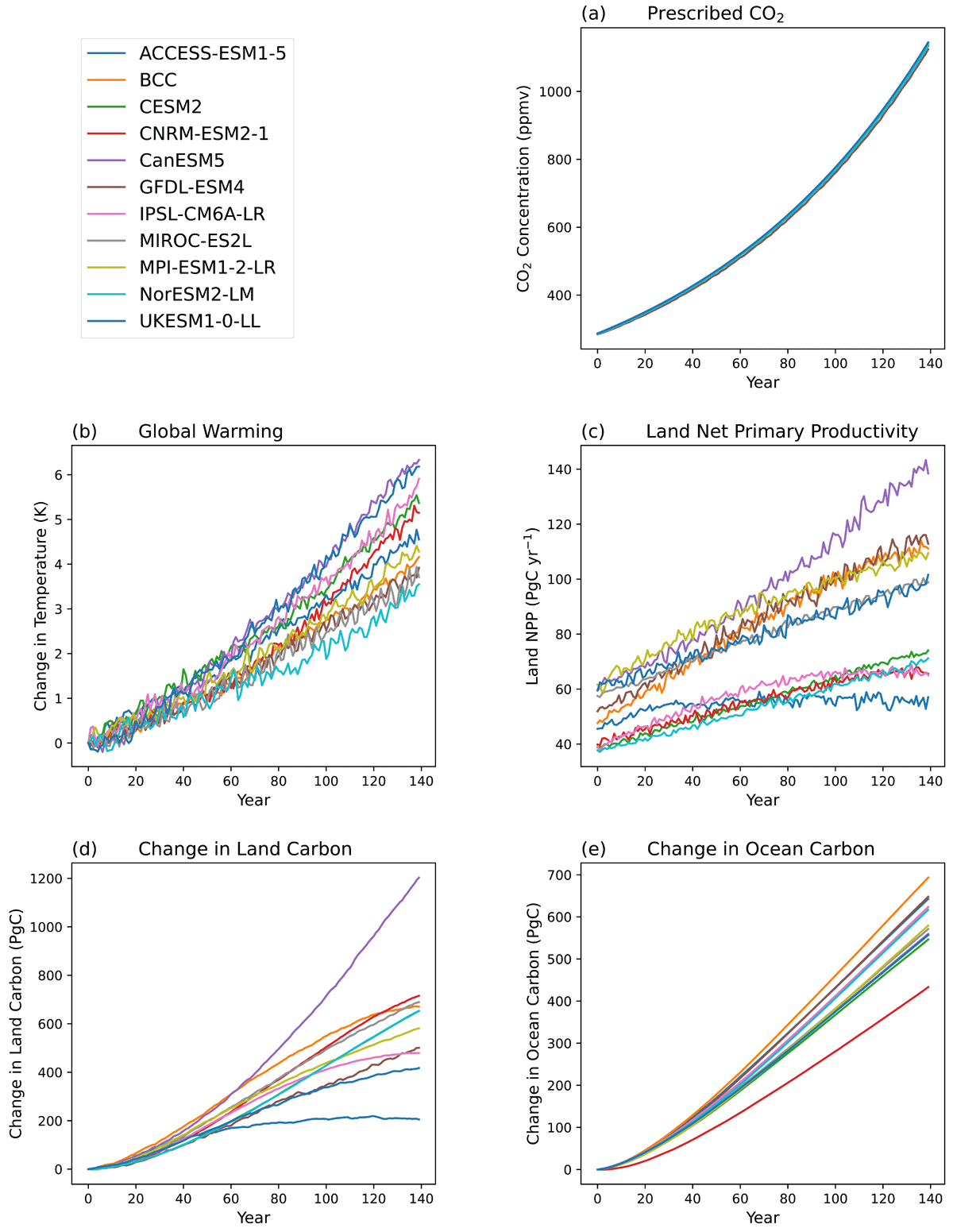
Figure 2
Global variables from the C4MIP coupled runs: (a) prescribed 1% per year increase in atmospheric CO2 concentration; (b) increase in global mean temperature; (c) global mean land net primary productivity; (d) change in land carbon storage; and (e) change in ocean carbon storage.
In order to reveal the sink saturation, we estimate the quasi-equilibrium state from Equation 5. Figure 3 shows the original transient BGC C4MIP runs (black lines), and this reconstructed quasi-equilibrium state (blue dots), with one panel for each of the C4MIP models. Now, ocean sink saturation is clearly seen in the reconstructed quasi-equilibrium of every model. We can now compare these quasi-equilibrium responses to the saturating CO2 response of Equation 6 using the estimated values of and . These reconstructions are shown by the blue lines in Figure 3 (and we do likewise for land carbon, see Supplementary Material, Figure S.4).
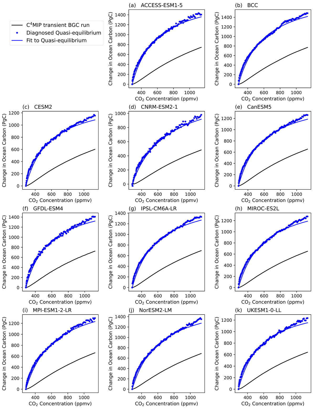
Figure 3
Fitting procedure for the CO2 response of the change in global ocean carbon storage, with a panel for each of the C4MIP models. Each panel shows the change in global mean ocean carbon from the C4MIP BGC run (black line); the quasi-equilibrium state inferred assuming a characteristic lifetime of 100 years in each model (blue dots); and our two-parameter fit to this quasi-equilibrium response (blue line).
Figure 4 shows a similar process for the climate response of land carbon. Here the climate response (shown by black dots) is diagnosed as the difference between the coupled runs (COU) and the BGC runs. We plot this residual against the temperature anomaly from the coupled run. In general, CO2-only responses are smoother (see Figure 3 for the ocean and Figure S.4 for the land), while climate-only responses show more scatter, especially for the land (see Figure 4 for the land and Figure S.5 for the ocean). However, all models show continuous reductions in the rate of land carbon uptake due to global warming, apart from CanESM5 for which the diagnosed climate change effect is negative to start with and then switches to become positive beyond a global warming of approximately 4C. As for ocean carbon uptake, models show evidence of lags in their responses, which introduces a curvature in the line linking the black dots (see Supplementary Material, Figure S.5). Again, we can estimate the quasi-equilibrium response using Equation 5 and the characteristic timescales diagnosed using Equation 4. The red dots in Figure 4 show this reconstructed quasi-equilibrium response for each model, which is always more linear in global warming than the transient response (black dots). The fitted straight line for the quasi-equilibrium response, with gradient , is also shown. We do likewise for for each model (Figure S.5).
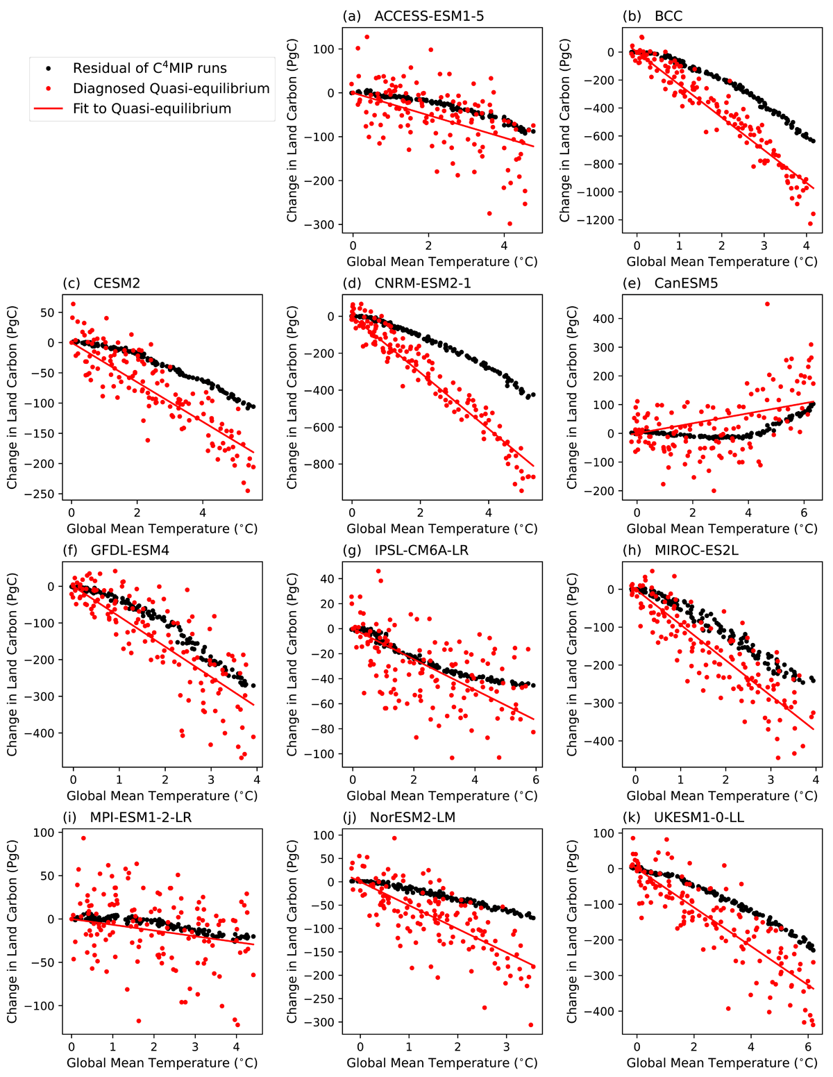
Figure 4
Fitting procedure for the climate response of global land carbon storage, with a panel for each of the C4MIP models. Each panel shows the change in global mean land carbon against global warming, calculated as the difference between the C4MIP BGC and coupled runs (black line); the quasi-equilibrium state inferred assuming a characteristic lifetime for land carbon in each model (red dots); and a linear fit to this quasi-equilibrium response (red line).
Table 2 shows the best-fit parameters for each model using our new method, and Figure S.6 compares the new and values with the old ones. It should be noted here that the parameters in the old and new approach are not directly comparable. In the new approach defines the initial sensitivity of the carbon store to CO2, from the pre-industrial CO2 concentration. In the old approach, relates to the mean impact of CO2 on the carbon stores from pre-industrial to 2×CO2 or 4×CO2. As a result of sink saturation, which is neglected in the standard approach, the new values are much larger. For the new approach, as with the old, we see more variation in the best-fit parameters for land carbon than for ocean carbon. Indeed, there is a good deal of model agreement on the ocean carbon responses to both CO2 and climate. For both land and ocean, it is notable that the new fit implies more negative land and ocean responses to global warming (ensemble mean moves from –4551 PgC/K to –6673 PgC/K; ensemble mean moves from –175 PgC/K to –4010 PgC/K). This is primarily due to fitting to diagnosed quasi-equilibrium states rather than the dynamical evolution of the carbon stores (see Figures 4 and S.5).
Figure 5 shows the fit of the new approach (thick dashed lines) to the changes in land and ocean storage in the coupled C4MIP runs (thick continuous lines). For comparison, we also show the old fits (thin continuous lines). It is clear that the new approach picks up the sink saturation effects that are evident in the C4MIP outputs but which cannot be captured by the linear approach. This is further evidenced by Figure 6, which shows root mean square errors (RMSEs) for the old and new approaches relative to the C4MIP outputs. With the single exception of the change in land carbon in CanESM5 (which is unusually linear when plotted against CO2), RMSEs are reduced significantly for all models and for both land and ocean, in the new approach. The improvement in the quality of the fit for land carbon uptake is especially impressive, with mean RMSE reduced by the new approach from about 70 PgC in the old approach, to about 17 PgC in the new.
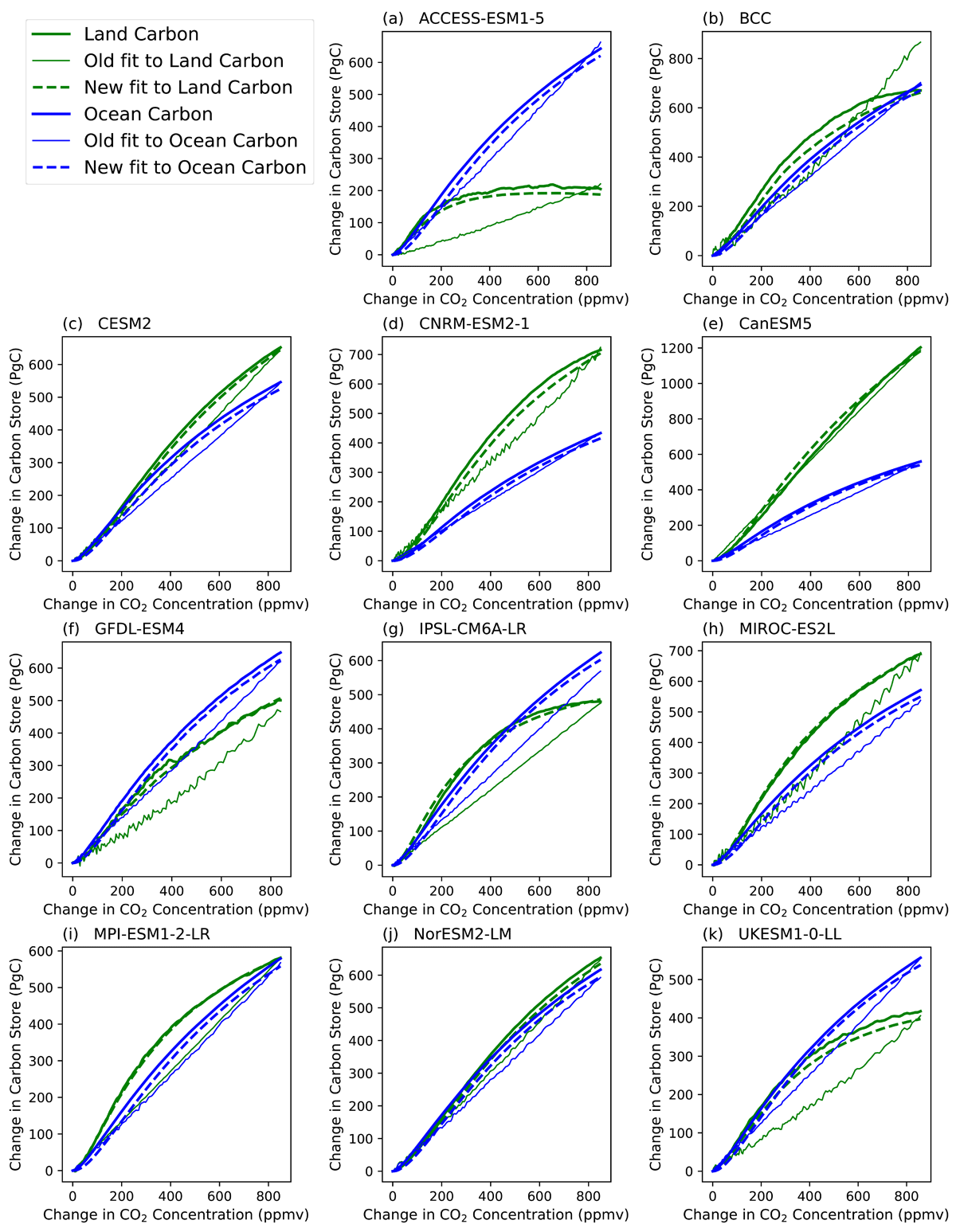
Figure 5
Comparison of fits to the change in land carbon storage (green lines) and ocean carbon storage (blue lines) for the coupled runs (thick continuous lines). Fits are shown for both the old model (thin continuous lines) and our new model (thick dashed lines).
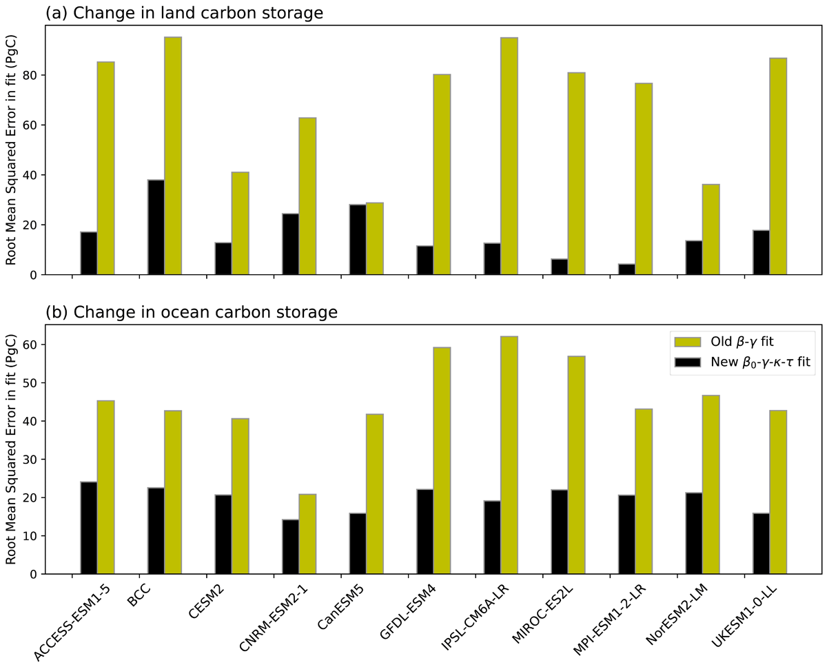
Figure 6
Root mean square errors in the fits of the old model (yellow bars), and the new model (black bars), for each of the C4MIP models: (a) change in land carbon; (b) change in ocean carbon.
4 Discussion
Our extension to the old model rests on four key assumptions. First, we assume that the quasi-equilibrium response can be reconstructed from the transient response using a single timescale. This assumption is more justifiable for land carbon than for ocean carbon, as ocean uptake is known to respond on multiple timescales (Canadell et al., 2021; Sarmiento and Toggweiler, 1984; Strassmann and Joos, 2018). To demonstrate this, we examine how well our new fit predicts the land and ocean carbon uptake 120 years after an abrupt quadrupling of CO2 (i.e., by examining the abrupt 4×CO2 runs with the C4MIP models). Figure S.7 shows that our fit to the 1% year runs does surprisingly well in predicting the land uptake in the 4×CO2 runs (see Figure S.7a). However, the assumption of a single timescale of the ocean response tends to overestimate carbon uptake 120 years after the abrupt CO2 increase (see Figure S.7b).
Second, we assume that the single timescale for land is approximated by the ratio of the equilibrium land carbon to the equilibrium NPP. The quality of the fits to the 1% per year runs (see Figure S.4), and the ability to approximately reproduce the abrupt 4×CO2 response (see Figure S.7a), suggest that this is a good assumption for the land. Thirdly, we assume that a single ocean timescale of 100 years is sufficient to identify the decadal-to-century timescale quasi-equilibrium response of the ocean. This is arguably the biggest weakness of our approach. It is an assumption that we have made in our attempt to develop a transparently simple extension to the existing formulation, but one that warrants further analysis in the future.
Finally, we assume that the quasi-equilibrium response to CO2 approximates a (Michaelis–Menton-like) hyperbolic response. The quality of the fit of the saturating hyperbolic to the diagnosed quasi-equilibrium from the CO2-only (BGC) runs suggests that this is a good assumption at least up to 900 ppmv for the ocean (see Figure 3), and for most land models up to 4×CO2 (see Figure S.4). The exceptions are ACCESS-ESM1.5 and IPSL-CM6A-LR, which show a loss of the quasi-equilibrium land carbon sink at high CO2 even in the absence of climate change effects. This may be indicative of these models having characteristic timescales that are not well approximated by the ratio of the equilibrium land carbon to equilibrium NPP.
Despite these simplifications within our new approach, it reproduces the C4MIP 1% per year runs much better than the existing approach without requiring any new runs to be analysed.
5 Conclusions
The carbon cycle and the climate system interact on timescales from seasonal to multi-millennial. Over the last 25 years, GCMs of the climate have started to include models of the land and ocean carbon cycle as interactive components. These models indicate that carbon cycle feedbacks on future climate change could be very important, but differences between models remain, especially in the response of the land carbon cycle to increases in CO2 and changes in climate. Reducing the remaining uncertainties will require a combination of better diagnosis, improvements in model process representation, and better model calibration. Until now, the diagnosis of the sources of differences between ESMs has relied on an assumption that changes in land and ocean carbon storage respond approximately linearly to changes in atmospheric CO2 and global warming (the ‘’ framework). In this paper, we have shown that the results from ESMs instead show strong evidence of sink saturation at high-CO2, which cannot be captured by the standard approach. We have therefore developed a simple extension to the existing approach to capture sink saturation and the characteristic timescales of carbon uptake by the land and ocean. The resulting provides a much improved fit to the outputs from complex coupled climate-carbon cycle GCMs. We hope that our new approach will be helpful in analysing the varying carbon cycle responses across different models, and between model generations. The representation of sink saturation effects within our approach should make it easier to identify the impact of new process representations such as nutrient limitations. In addition, it is vital to keep sink saturation in mind when considering future carbon sinks, and our new approach allows these effects to be much more clearly diagnosed.
Code availability
Code accompanying this paper can be found on GitHub at https://github.com/josephjclarke/ClimateCarbonCycleFeedbacks
Additional File
The additional file for this article can be found as follows:
Data availability
The CMIP6 Earth system model output data is available online: https://esgf-node.ipsl.upmc.fr/projects/cmip6-ipsl/ and the C4MIP data used in Arora et al. (2020) is available at: https://c4mip.net/results.
Author Contributions
PMC conceived of the new approach and designed the study. JJC processed the C4MIP models data and drafted Section 3. SJ drafted Section 1 and RMV drafted Section 2 of the paper. All authors contributed to the study and to the submitted paper.