
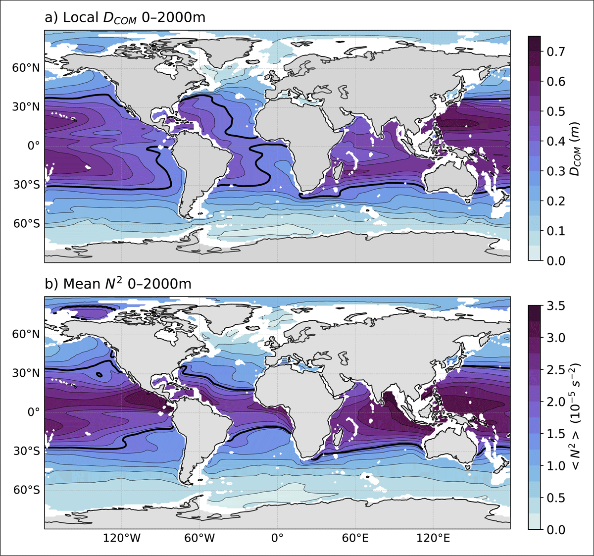
Figure 1
Spatial distribution of the time-mean (a) DCOM (in m), and (b) mean-N2 (in ) computed for the upper 2000 m of each horizontal grid points at location deeper than 2000 m. Estimated using the ECCOv4r4 for the period 1992–2017 (see Method section). The thick black contour corresponds to the corresponding global mean value, highlighting important local differences between the spatial distributions of the two indices. Regions shallower than 2000 m were masked (white).
Table 1
Short correspondence table for a given control volume (V in z-coordinates, in p-coordinates). In all cases, (with the appropriate averaging operator). Notation: S is Absolute Salinity, is Conservative Temperature, is in-situ density, is a constant reference density, is specific volume, is potential density anomaly (referenced to the surface), is PEA, b is buoyancy defined as , z is height (positive upward) and p is pressure; and are the corresponding reference levels; angle brackets denote a volume average over V, and a pressure-coordinate volume average over ; and are dynamic enthalpies as defined in the table, and the subscript 0 denotes the fully mixed reference state obtained by replacing by their corresponding volume means over the same control volume.
| POT. DENSITY APPROX. | BOUSSINESQ APPROX. | COMPRESSIBLE FLUID | |
|---|---|---|---|
| “Vertical” coordinate | Height z | Height z | Pressure p |
| Infinitesimal volume | |||
| “Volume” average | |||
| Reference level | |||
| Effective PE (local) | |||
| Fully-mixed PE (local) | |||
| Depth anomaly | |||
| Mean- |
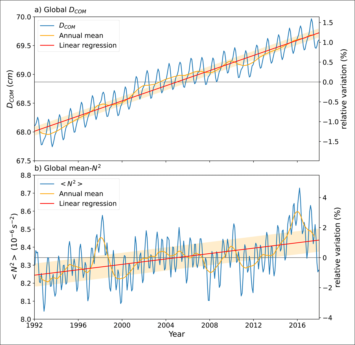
Figure 2
Time series of (a) global DCOM (in cm), and (b) global mean-N2 (in ). Plots include monthly mean (blue) and the associated linear regression line (red) with an envelope representing the standard error (shaded orange). The annual mean is superimposed (orange). Corresponding variations relative to the mean are indicated on the right axis.
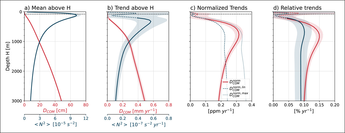
Figure 3
Distribution of (a) mean (), (b) trends (), (c) normalized trends (), and (d) relative trend () of stratification indices as a function the maximum depth H of the considered ocean volume. In the four panels, the depth anomaly DCOM is shown in red and the mean-N2 in blue. Trends that are not statistically significant are dashed (based on p-value for a Kendall’s tau test (Kendall, 1938). The mean depth of the ocean volume shallower than H is used to normalize trends in (c). The depth of global mean mixed layer is indicated with the vertical dashed black line.
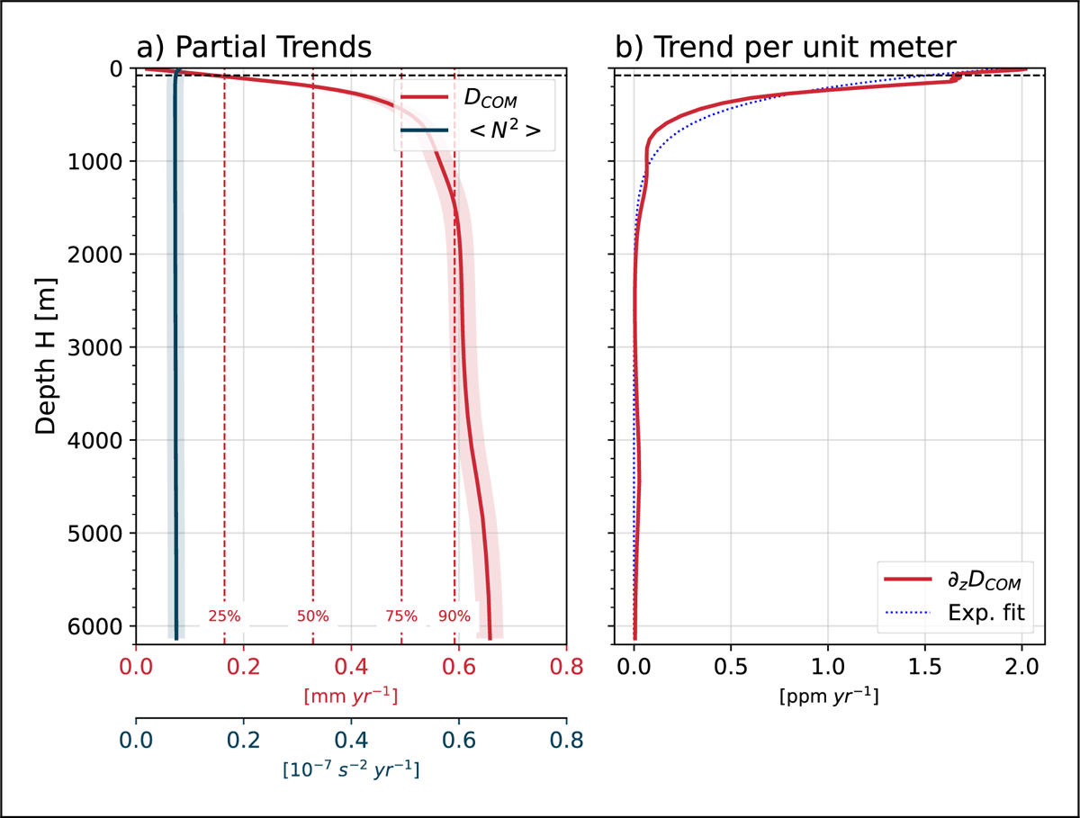
Figure 4
Distribution of (a) DCOM and mean-N2 partial trends (), and (b) DCOM partial trends per unit depth as a function of depth H. Partial trends are obtained on the full volume of the ocean, when the properties deeper than H have been time-averaged. Horizontal dashed red lines in (a) show DCOM that are 25%, 50%, 75%, and 90% of the global trend. The dashed blue line indicates an exponential fit of partial trends per unit depth in (b). The global-mean mixed layer depth is indicated with a dashed black line.
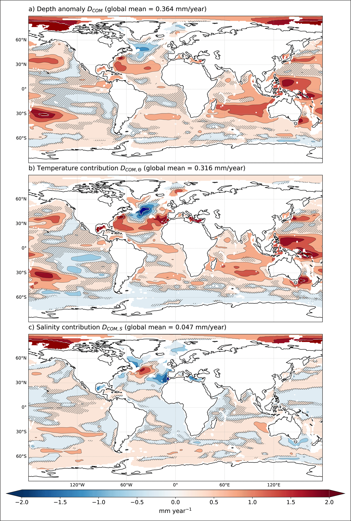
Figure 5
Spatial patterns of the 0–2000 m stratification trends, based on (a) DCOM, (b) , and (c) DCOM,S. Linear trends are computed for the 1992–2017 period. Values are given in mm per year, where positive values indicate enhanced stratification and negative values indicate weakened stratification. A 0.5 mm yr–1 contour interval is used. The stippling in (a–c) indicates regions that are not statistically significant at 90% confidence. On average, the depth anomaly is increasing at an average rate of 0.36 mm yr–1, but local trend values can be more than 10 times larger in certain areas.
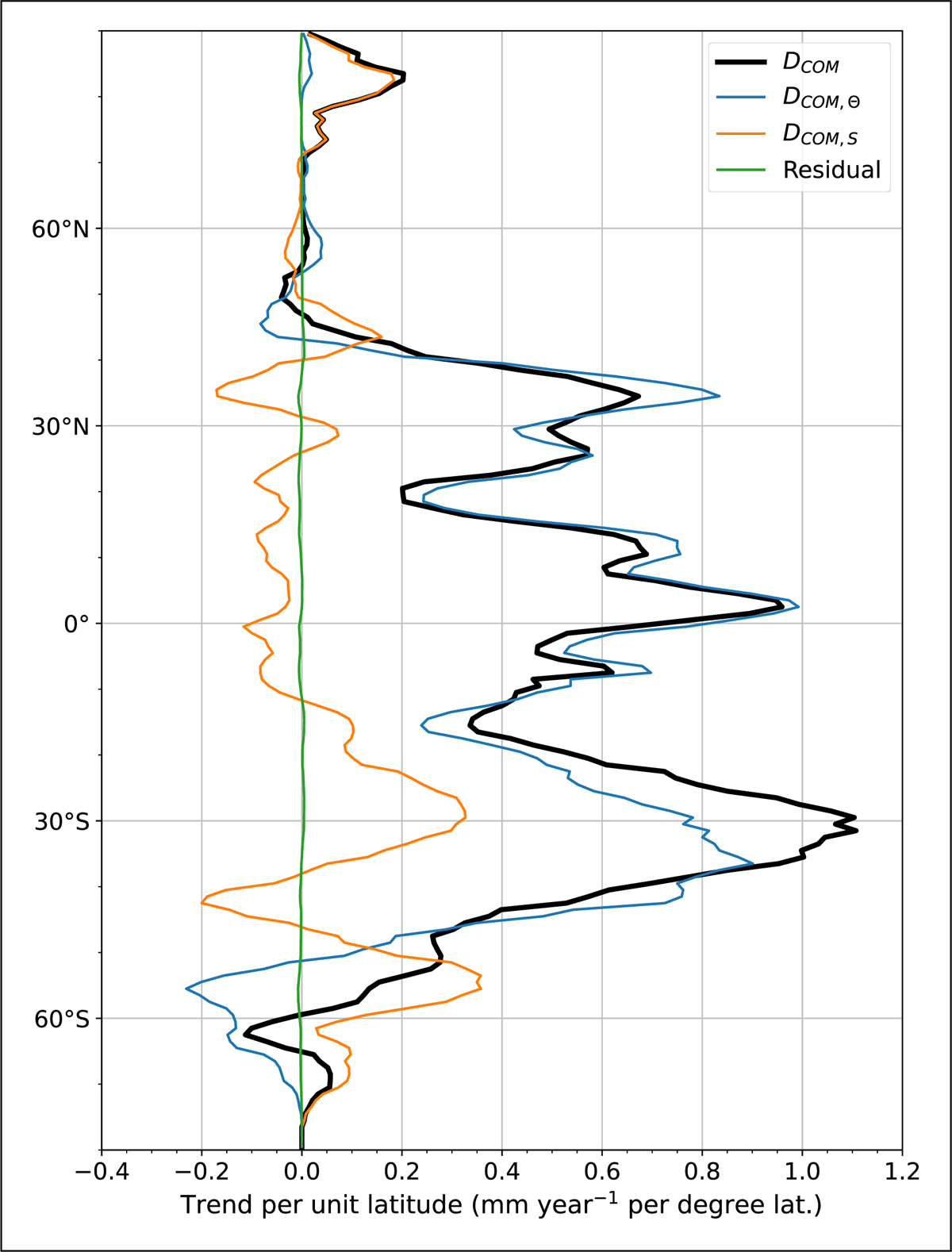
Figure 6
Zonally averaged trends of local depth anomaly for the upper 2000 m water column DCOM, and the respective contribution from temperature , and salinity DCOM,S. The residual DCOM minus is negligible at all latitudes. Trends are scaled by the total area of open ocean (i.e., deeper than ) per unit latitude.
Table 2
Mean, trend, relative trend, and SE of the relative trend are tabulated for the two stratification indices (depth anomaly and mean-N2), considering ocean volumes for different depth ranges.
| GLOBAL MEAN | 0–207 m | 0–513 m | 0–958 m | 0–1993 m | FULL DEPTH | |
|---|---|---|---|---|---|---|
| DCOM | Mean (cm) | 3.52 | 10.29 | 19.08 | 35.32 | 68.87 |
| Trend (mm y-1) | 0.01 | 0.13 | 0.28 | 0.39 | 0.66 | |
| Relative Trend (% year-1) | 0.03 | 0.13 | 0.15 | 0.11 | 0.10 | |
| SE of the relative trend (% year-1) | 0.023 | 0.009 | 0.005 | 0.003 | 0.002 | |
| mean-N2 | Mean (10-5 s-2) | 9.08 | 4.93 | 2.86 | 1.52 | 0.75 |
| Trend (10-8 s-2 year-1) | 3.57 | 4.93 | 2.86 | 1.52 | 0.75 | |
| Relative Trend (% year-1) | 0.04 | 0.10 | 0.10 | 0.09 | 0.09 | |
| SE of the relative trend (% year-1) | 0.019 | 0.013 | 0.011 | 0.010 | 0.009 |
Table 3
Spatial correlations between various local trends.
| DCOM | mean-N2 | |
|---|---|---|
| Buoyancy anomaly (0–2000 m) | 0.857 | 0.573 |
| Heat anomaly (0–2000 m) | 0.462 | 0.192 |
| Salt anomaly (0–2000 m) | –0.314 | –0.314 |
| Surface buoyancy | 0.451 | 0.691 |
| Surface temperature | 0.384 | 0.408 |
| Surface salinity | -0.188 | -0.441 |
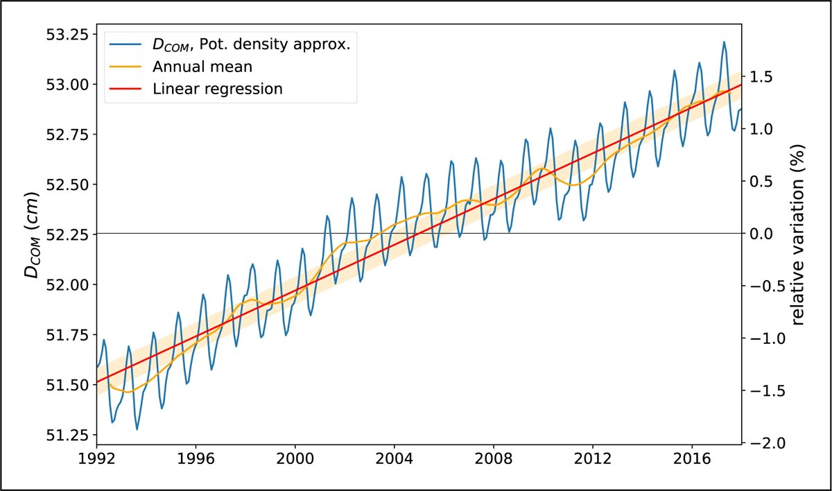
Figure A.1
Time series of global DCOM computed using the potential density approximation (see Table 1). As in Figure 2, the linear regression line (red) is shown with an envelope representing ± the standard error (shaded orange), and the annual mean is superimposed (orange). Corresponding variations relative to the mean are indicated on the right axis.