
1 Introduction
Ocean stratification is an important control for exchanges of heat, carbon, and nutrients between the surface and the deep ocean (Bopp et al., 2013; Cheng et al., 2025; Wunsch and Ferrari, 2004). The ongoing climate changes, which are mostly driven by anthropogenic release of greenhouse gases such as carbon dioxide (IPCC, 2019), have generated a global warming in the last decades, which is expected to strengthen ocean stratification (Capotondi et al., 2012) and affect the global ocean circulation, with important consequences for marine life and ocean currents (Bindoff et al., 2019). Ocean stratification can be directly linked to ocean de-oxygenation and reduced ventilation (Breitburg et al., 2018), and it is affecting the abundance and distribution of marine species (Venegas, Acevedo and Treml, 2023).
It has been recently estimated that the global stratification in the upper 2000 m has increased by 5.3% since 1960, or 0.9% per decade (Li et al., 2020). Similarly, Yamaguchi and Suga (2019) found a global increase of 3.3–6.1% in the upper 200 m with significant spatial variability, or 0.6–1.1% per decade. Repeating the analysis of Li et al. (2020), Cheng et al. (2024) found a record high stratification in 2023, corresponding to record high sea surface temperature (SST) at the time of publication. These estimates, used in the IPCC report (IPCC, 2019), are all based on depth averages of the squared buoyancy frequency.
The squared buoyancy frequency N2 is a standard measure of the local stratification,
where is the in situ density, g the gravity acceleration, and z the height increasing upward. The mean squared buoyancy frequency (mean-N2) then appears as a natural way to measure the stratification of a control volume,
where the brackets denote a volume average.
The mean-N2 has been used to study stratification changes using localized water columns over various depth ranges as control volume. The depth H over which N2 was averaged varied according to studies, with m (Cheng et al., 2024; Li et al., 2020) or m (Capotondi et al., 2012; Li et al., 2020) being common choices. Other studies focused on the 15 m immediately below the mixed layer (Roch, Brandt and Schmidtko, 2023; Sallée et al., 2021) or used a phenomenological model of vertical stratification to determine the pycnocline depth range (Somavilla et al., 2026). These estimates are more uncertain due to the difficulty in determining the mixed layer depth and pycnocline characteristics (Cheng et al., 2025).
The mean-N2 index has, however, some limitations, due to its high sensitivity to variability at endpoints. The mean-N2 value for a water column of depth H is indeed approximately proportional to the top-to-bottom density difference,
where is the surface-referenced potential density anomaly and a constant reference density (often taken as kg m-3). As the ocean variability increases by several orders of magnitude at the surface, the mean-N2 tends to be strongly affected by seasonal and shorter-term variability in the surface layer. Furthermore, this index does not feel changes in the shape of density profiles between the surface and the depth H, such as a deepening of the pycnocline would produce.
The depth anomaly measures how much the center of mass (COM) is deeper relative to a fully mixed reference state (Rosenthal and Roquet, 2025),
where is a local measure of potential energy, and the associated potential energy of the mixed state. It is by definition proportional to the total work that would be required to fully mix a given control volume (the global ocean, a horizontal slab, a water column…), making it positive for a stably stratified ocean, and exactly zero for an unstratified state (as is also the mean-N2). Following Rosenthal and Roquet (2025), we use dynamic enthalpy instead of potential energy to define the COM. This implies that the definition of the COM used here differs slightly from the mass-weighted mean depth in a way that better accounts for compressibility effects.
Visual inspection of the global maps of mean-N2 and DCOM for the upper water column illustrates the fundamental differences (Figure 1). Overall, both indices show a stronger stratification in lower latitudes as expected. However, while the mean-N2 reaches its maximum in the tropics, in line with the SST, the depth anomaly of the COM is deepest in the subtropical gyres with a distribution that better resembles vertically integrated quantities such as the ocean heat content (OHC). It also shares a remarkable similarity with the spatial distribution of the sea surface height (SSH).
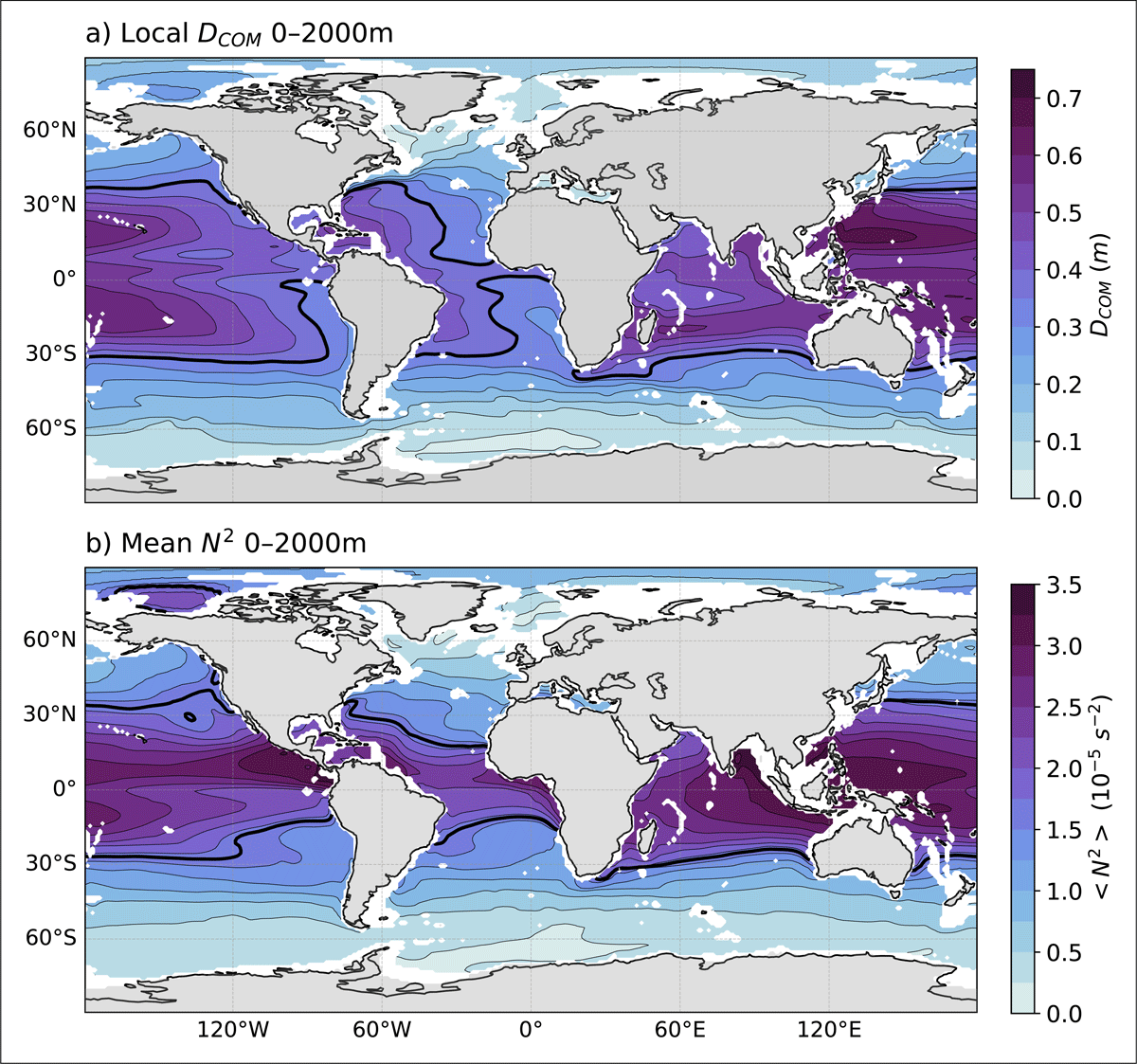
Figure 1
Spatial distribution of the time-mean (a) DCOM (in m), and (b) mean-N2 (in ) computed for the upper 2000 m of each horizontal grid points at location deeper than 2000 m. Estimated using the ECCOv4r4 for the period 1992–2017 (see Method section). The thick black contour corresponds to the corresponding global mean value, highlighting important local differences between the spatial distributions of the two indices. Regions shallower than 2000 m were masked (white).
Note that the depth anomaly is approximately proportional to the potential energy anomaly (PEA), a concept initially proposed by Simpson (1981), and which is often used to study stratification changes in various regional contexts (Burchard and Hofmeister, 2008; Dörr et al., 2024; Marsh et al., 2024; Muilwijk et al., 2023; Yamaguchi et al., 2019). Using , the depth anomaly is approximately,
where is the PEA. This approximation is accurate for shallow water columns ( m), but it neglects compressibility effects that can become important in deeper water columns (see Appendix A). In this sense, the depth anomaly can be seen as a generalization of PEA.
The purpose of this paper is to investigate stratification changes, computing global and local trends of the mean-N2 and DCOM indices in the Estimating the Climate and Circulation of the Ocean (ECCO) product, which provides an observationally constrained ocean state estimate for the 26-year long period 1992–2017. We will also analyze how results based on mean-N2 and DCOM differ, how local trends depend on the choice of water column depth range, and quantify the relative contribution of temperature and salinity on the observed trends.
2 Definitions
2.1 Depth anomaly
The depth anomaly DCOM measures how much the COM is lowered due to the stratification, compared with a fully mixed state (Rosenthal and Roquet, 2025). We provide three definitions (see Table 1), the first neglecting compressibility effect in the equation of state, the second retaining them but making the Boussinesq approximation (no volume expansion), and the third being the most accurate as it accounts for both compressibility and expansion effects (compressible case).
Table 1
Short correspondence table for a given control volume (V in z-coordinates, in p-coordinates). In all cases, (with the appropriate averaging operator). Notation: S is Absolute Salinity, is Conservative Temperature, is in-situ density, is a constant reference density, is specific volume, is potential density anomaly (referenced to the surface), is PEA, b is buoyancy defined as , z is height (positive upward) and p is pressure; and are the corresponding reference levels; angle brackets denote a volume average over V, and a pressure-coordinate volume average over ; and are dynamic enthalpies as defined in the table, and the subscript 0 denotes the fully mixed reference state obtained by replacing by their corresponding volume means over the same control volume.
| POT. DENSITY APPROX. | BOUSSINESQ APPROX. | COMPRESSIBLE FLUID | |
|---|---|---|---|
| “Vertical” coordinate | Height z | Height z | Pressure p |
| Infinitesimal volume | |||
| “Volume” average | |||
| Reference level | |||
| Effective PE (local) | |||
| Fully-mixed PE (local) | |||
| Depth anomaly | |||
| Mean- |
We describe now the definition for the seawater Boussinesq case, as in Rosenthal and Roquet (2025). The depth anomaly is function of the Boussinesq dynamic enthalpy (Young, 2010), defined as,
Here, is the buoyancy function of absolute salinity S, conservative temperature and an approximate sea pressure p proportional to the height z, following the TEOS-10 standard (Roquet et al., 2015). The Boussinesq dynamic enthalpy is defined relative to a reference height z0, generally taken as the mean sea level. It is, however, straightforward to compute it for any reference level z1, as the difference .
We now consider a control volume V onto which we want to compute the depth anomaly. The depth anomaly is proportional to the difference in volume-averaged dynamic enthalpy between the control volume and the corresponding fully mixed volume (with volume-averaged conservative temperature and absolute salinity),
Importantly, dynamic enthalpies are computed relative to the center of volume, defined as the average height over the control volume (Rosenthal and Roquet, 2025).
The depth anomaly can be defined for any control volume, providing a lot of flexibility in its use. We define in particular the global depth anomaly as the depth anomaly for the full volume of the ocean (see Figure 2). A local depth anomaly can also be defined for water columns of given depth range, to generate spatial maps as in Figure 1. The sensitivity to the choice of depth range is illustrated in Figure 3, and the contribution per depth to stratification change is diagnosed in Figure 4.
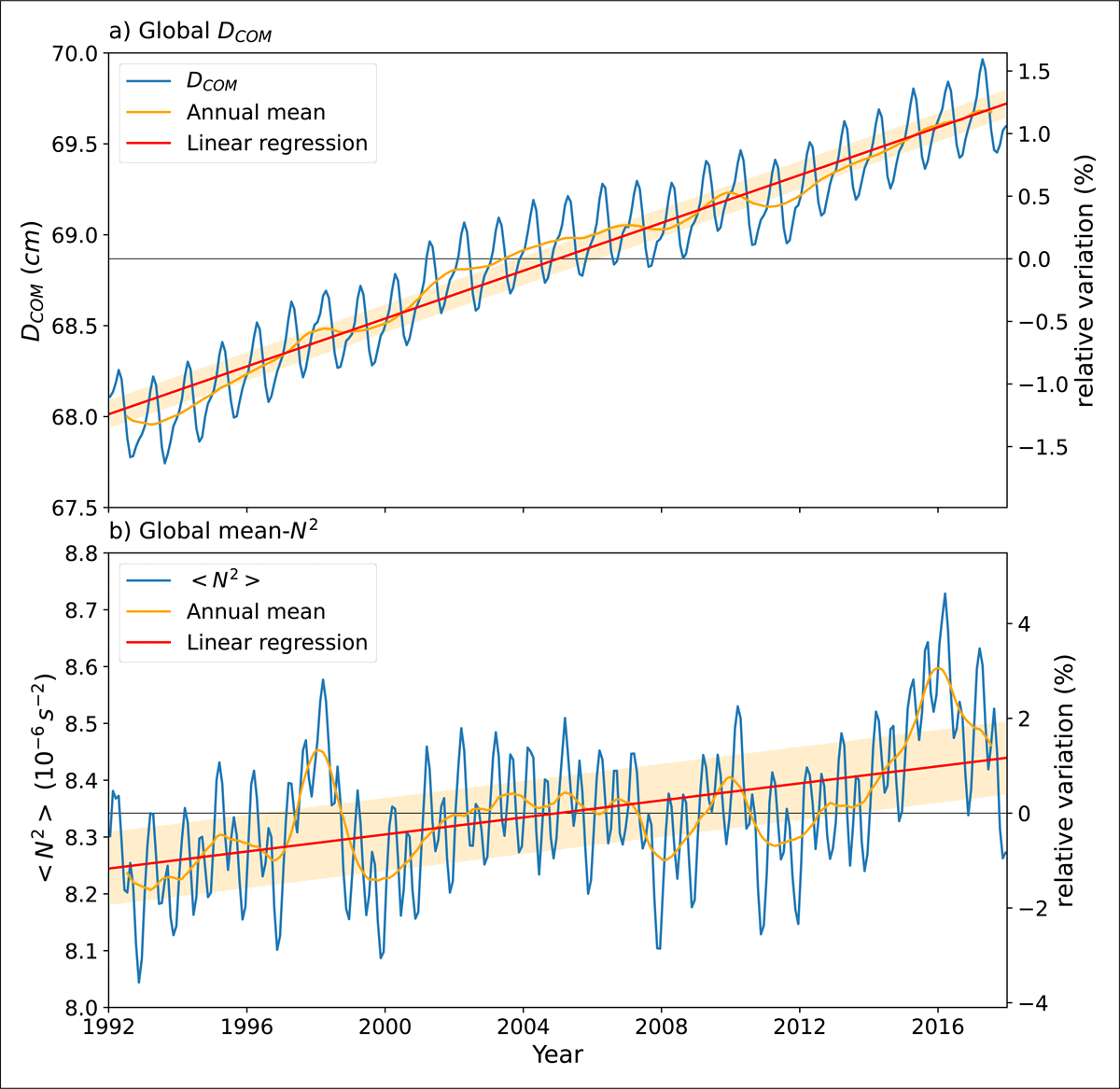
Figure 2
Time series of (a) global DCOM (in cm), and (b) global mean-N2 (in ). Plots include monthly mean (blue) and the associated linear regression line (red) with an envelope representing the standard error (shaded orange). The annual mean is superimposed (orange). Corresponding variations relative to the mean are indicated on the right axis.
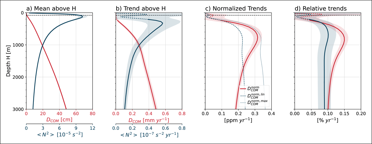
Figure 3
Distribution of (a) mean (), (b) trends (), (c) normalized trends (), and (d) relative trend () of stratification indices as a function the maximum depth H of the considered ocean volume. In the four panels, the depth anomaly DCOM is shown in red and the mean-N2 in blue. Trends that are not statistically significant are dashed (based on p-value for a Kendall’s tau test (Kendall, 1938). The mean depth of the ocean volume shallower than H is used to normalize trends in (c). The depth of global mean mixed layer is indicated with the vertical dashed black line.
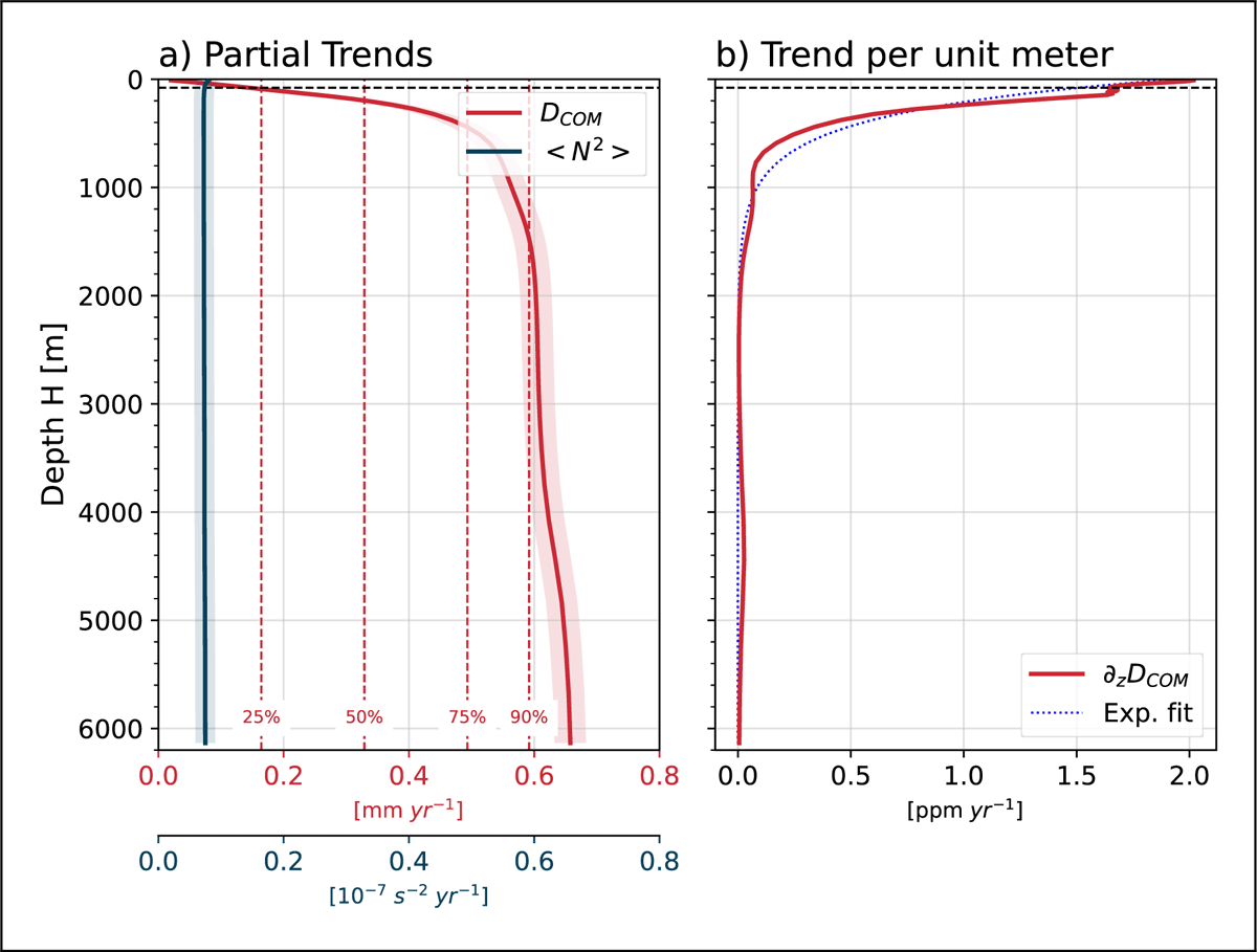
Figure 4
Distribution of (a) DCOM and mean-N2 partial trends (), and (b) DCOM partial trends per unit depth as a function of depth H. Partial trends are obtained on the full volume of the ocean, when the properties deeper than H have been time-averaged. Horizontal dashed red lines in (a) show DCOM that are 25%, 50%, 75%, and 90% of the global trend. The dashed blue line indicates an exponential fit of partial trends per unit depth in (b). The global-mean mixed layer depth is indicated with a dashed black line.
2.2 Comparison with mean-N2
It is interesting to compare the depth anomaly with the mean-N2 for simple density profiles to better understand their differences. Assume a linear stratification, for which N2 is constant. Neglecting compressibility effects, the depth anomaly simplifies to (see Appendix B). In fact, the depth anomaly for a given value of mean-N2 ranges between zero for an infinitesimally thin density jump at the surface or at the bottom, and for a two-layer profile with equal depths. This illustrates how the shape of the density profile may affect the stratification despite having no signature on the mean-N2 index.
These considerations give a natural way to normalize and compare both indices. The depth anomaly can be normalized by the water column depth, , while the mean-N2 can be translated into what the normalized depth anomaly would be if the stratification was linear, , or as the maximum normalized depth anomaly, (see Figure 3c).
2.3 Temperature and salinity contributions
Relative contributions of temperature and salinity to the depth anomaly can be estimated by introducing two partially mixed reference states, in which only one tracer is homogenized while the other is left unchanged. Specifically, the state isolates the contribution of temperature anomalies at fixed mean salinity, whereas isolates the contribution of salinity anomalies at fixed mean temperature. Using the fully mixed reference state , we define
This construction is consistent with a first-order linearization of about the fully mixed state : to leading order, the dependence on S and separates, so that recovers DCOM. The decomposition is therefore exact for a linear equation of state, while any residual reflects nonlinear effects (including S– interaction terms and pressure-dependent nonlinearities). In practice, the discrepancy between and the full DCOM is small, as illustrated in Figures 5 and 6.
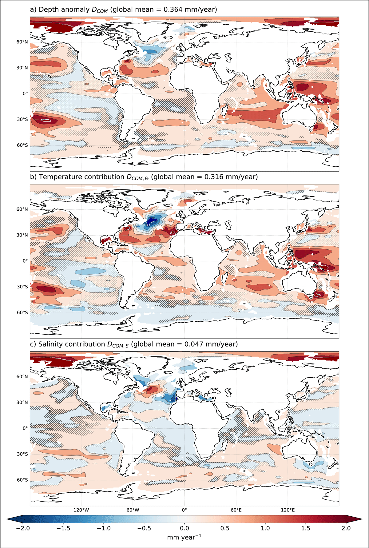
Figure 5
Spatial patterns of the 0–2000 m stratification trends, based on (a) DCOM, (b) , and (c) DCOM,S. Linear trends are computed for the 1992–2017 period. Values are given in mm per year, where positive values indicate enhanced stratification and negative values indicate weakened stratification. A 0.5 mm yr–1 contour interval is used. The stippling in (a–c) indicates regions that are not statistically significant at 90% confidence. On average, the depth anomaly is increasing at an average rate of 0.36 mm yr–1, but local trend values can be more than 10 times larger in certain areas.
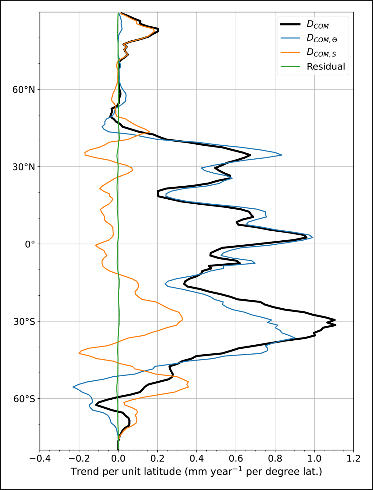
Figure 6
Zonally averaged trends of local depth anomaly for the upper 2000 m water column DCOM, and the respective contribution from temperature , and salinity DCOM,S. The residual DCOM minus is negligible at all latitudes. Trends are scaled by the total area of open ocean (i.e., deeper than ) per unit latitude.
2.4 Compressible case
The known isomorphism between the seawater Boussinesq model and the hydrostatic compressible model in pressure coordinates offers a straightforward way to generalize the depth anomaly definition (Marshall et al., 2012; Roquet, 2013), using pressure as vertical coordinate instead of height. We provide the generalized definitions in Table 1 for completeness. This definition gives nearly identical results for the quasi-incompressible ocean, but opens up potential applications to study the highly compressible atmosphere.
This generalization also helps elucidate how fluid expansion affects the depth anomaly. If one considers a column of fluid that is heated homogeneously, the COM of the column is raised as the fluid expands. This would not affect the COM when making the Boussinesq approximation; however, it does for a compressible ocean. However, the fluid “volume” remains constant in pressure coordinates and the generalized COM remains unchanged. In other words, steric effects do not change the control volume, and they change the depth anomaly only when they are associated with a stratification change through differential heating in the vertical.
On the other hand, adding fluid on top of the column raises the COM at nearly the same rate as it raises the COM of the mixed state. The discrepancy depends on the density difference of the added volume compared to the mixed state. Thus, the depth anomaly remains virtually unchanged as long as the volume-averaged temperature and salinity vary little, as is always the case in the ocean.
3 Method
3.1 ECCO product
The analysis is carried out on the ocean state estimate ECCO version 4 Release 4 (ECCOv4r4, https://www.ecco-group.org). The ECCO state estimate is obtained from a MITgcm global configuration, solving numerically the hydrostatic Boussinesq equations (Forget et al., 2015), while using an inverse method to adjust the initial state, forcing fields, and mixing parameters. This method allows the solution to remain close to most available satellite and in situ observations, while avoiding the introduction of non-conservative perturbations to the model run (Wunsch, Williamson and Heimbach, 2023). Monthly averaged fields of temperature and salinity are provided on a global 1° resolution grid with 50 vertical levels (Fukumori et al., 2021). The product is available for a 26-year-long period (1992–2017).
The model MITgcm uses the Boussinesq approximation, so the depth anomaly is defined using the Boussinesq dynamic enthalpy, following Equ. (7). The function gsw_dynamic_enthalpy in the TEOS-10 toolbox1 provides the dynamic enthalpy (enthalpy minus potential enthalpy) referenced to a referenced surface pressure () as a function of absolute salinity, conservative temperature, and pressure. A linear conversion between pressure and height is used for the pressure input. The Boussinesq dynamic enthalpy referenced to a given center of volume zv is then approximated as .
Note that the MITgcm configuration used to compute the ECCOv4r4 state estimate does not implement the TEOS-10 equation of state, but a modified version of EOS-80 (Jackett and Mcdougall, 1995). However, following recommendations of McDougall et al. (2021), we chose to interpret ECCOv4r4 outputs as absolute salinity and conservative temperature regardless of the actual equation of state implemented in the model. Consequently, we use the TEOS-10 official definition of dynamic enthalpy in our computations (Roquet et al., 2015).
3.2 Temporal trends
Linear trends are calculated on timeseries of DCOM and mean-N2 (Figure 2). Trends are divided by the associated time mean to obtain relative trends. Uncertainty is estimated using twice the standard error (SE) of the trend. Trends were considered significant at 90% confidence when the p-value of the non-parametric Kendall coefficient was lower than 0.1 (Kendall, 1938) for global (Figure 3) and local trends (Figures 5 and 6).
Mean, trends, and relative trends are tabulated for different volumes of the ocean ranging from the surface to given depths H, and their relation to the maximum depth range is shown in Figure 3. This helps elucidate the sensitivity of trend estimates to the considered depth range.
Another computation is done to determine at which depth density changes contribute the most to the observed stratification trends. This is analyzed by considering global trends of DCOM and mean-N2 (from surface to bottom), obtained once temperature and salinity below a given depth H have been time-averaged. This provides a vertical profile of trends generated by density changes above the variable depth H. Taking the vertical derivative of this vertical profile gives the contribution to the observed trend by unit depth.
Correlations between various timeseries are computed using Pearson correlation coefficients. Timeseries include global mean SST, global mean surface buoyancy, and OHC. Only statistically significant correlations (at 90% confidence) are reported. Spatial patterns are also analyzed between local trends computed from upper 2000 m water columns. Area-weighted correlations between linear trends are computed for the two indices, and compared with vertically integrated anomalies of buoyancy, heat, and salt, as well as with surface buoyancy, temperature, and salinity (Table 3).
4 Results
4.1 Timeseries and global trends
The global depth anomaly of the COM (Figure 2a) presents a clear upward trend, indicative of a stratification increase in the last 26 years. During the ECCOv4r4 period, the depth anomaly has increased by nearly 2 cm, which represents a relative increase of 1% per decade (Table 2). The timeseries present a clear seasonal variability of amplitude 3 mm that can be attributed to the larger ocean area in the southern hemisphere than in the northern, but interannual variability is barely visible with deviations relative to the linear regression line of order 1 mm.
Table 2
Mean, trend, relative trend, and SE of the relative trend are tabulated for the two stratification indices (depth anomaly and mean-N2), considering ocean volumes for different depth ranges.
| GLOBAL MEAN | 0–207 m | 0–513 m | 0–958 m | 0–1993 m | FULL DEPTH | |
|---|---|---|---|---|---|---|
| DCOM | Mean (cm) | 3.52 | 10.29 | 19.08 | 35.32 | 68.87 |
| Trend (mm y-1) | 0.01 | 0.13 | 0.28 | 0.39 | 0.66 | |
| Relative Trend (% year-1) | 0.03 | 0.13 | 0.15 | 0.11 | 0.10 | |
| SE of the relative trend (% year-1) | 0.023 | 0.009 | 0.005 | 0.003 | 0.002 | |
| mean-N2 | Mean (10-5 s-2) | 9.08 | 4.93 | 2.86 | 1.52 | 0.75 |
| Trend (10-8 s-2 year-1) | 3.57 | 4.93 | 2.86 | 1.52 | 0.75 | |
| Relative Trend (% year-1) | 0.04 | 0.10 | 0.10 | 0.09 | 0.09 | |
| SE of the relative trend (% year-1) | 0.019 | 0.013 | 0.011 | 0.010 | 0.009 |
In contrast, the global mean-N2 presents a large interannual variability over the considered period. This variability correlates well with the El Nino Southern Oscillation, with very large maxima in 1998 and 2016, and important minima (La Nina events) in 2000, 2008, and 2012 (Alizadeh, 2024). As for the depth anomaly, the mean-N2 signal presents a significant seasonal variability, of amplitude s-2 or more. Superimposed on this seasonal and interannual variability, a significant upward trend of s-2 can be seen, which represents a 0.9% relative increase per decade. Note that the good match between the relative trends of the two indices should not be regarded as self-evident. The ratio between these two metrics is not fixed in general, as it relates to the vertical distribution of density. This suggests that overall, the shape of the stratification has not changed significantly during the ECCOv4r4 period.
While the relative trends are comparable for the two indices (~1% per decade), the signal-to-noise ratio is much higher for the depth anomaly index than for the mean-N2 index (SE of relative trend 5x smaller, Table 2). Also, the depth anomaly shows that the stratification has been increasing far more steadily over the 26-year-long period of ECCO than suggested by the mean-N2 index.
4.2 Comparing trends for different depth ranges of water column
Any stratification index must depend on the depth range considered. Various numbers exist in the literature, but they can be hard to interpret or to compare as they are often given for water columns of different depth ranges. Here, we explore more systematically the dependence of stratification index on the maximum depth H of the considered water volume (Figure 3, Table 2).
Stratification as measured by mean-N2 is generally maximal right below the mean mixed layer depth and decreases rapidly in the upper thermocline of the water column. The mean-N2 index then varies in at depth (Figure 3a), as expected from a stratification dominated by shallow density changes. By contrast, the depth anomaly is proportional to how much work is required to fully mix the considered ocean volume. It must therefore increase monotonously with H, in a nearly linear fashion at depth.
Similarly, linear trends of the two indices have a markedly different variation with depth range (Figure 3b). The mean-N2 experiences the fastest trend when considering the upper 300 m only, and then decreases with increasing H. The fastest trend in depth anomaly is obtained when considering the full ocean volume, reflecting the fact that its values increase quasi-linearly with H.
A better way to compare the two indices is to normalize their values (Figure 3c). The depth anomaly is naturally normalized by the considered depth H, with trends measured in part per million (ppm) per year. The maximum normalized trend is obtained for a depth , with a value close to what a two equal-depth layer would have (Appendix A). The normalized trend then decreases with depth and intersects the value for a linear stratification at a depth . This behavior indicates that most stratification changes must be concentrated in the upper 350 m. As one increases H, the stratification becomes comparatively shallower and the depth anomaly decreases relative to its maximum and linear values (Appendix A).
Both indices show results sensitive to the maximum depth H, and associated with large depth range dependence for layers shallower than m. This casts doubt on the robustness of shallow estimates, such as those solely based on the upper 200 m (at least for global estimates) that are very common in the literature (Cheng et al., 2025).
Normalizing the trends by the mean values, one obtains a relative trend index (Figure 3d). The maximum in relative trend of the depth anomaly is 0.15%/year, obtained when considering the upper 800 m volume. The depth anomaly value then decreases to stabilize around 0.1%/year for depth ranges reaching deeper than 2000 m. This justifies a posteriori the common use of 0–2000 m depth range to assess global stratification changes. The relative trend of the mean-N2 index stabilizes faster around a similar 0.1%/year value for layers deeper than m. The estimate is, however, associated with larger uncertainties, and as pointed out earlier, the correspondence between the two relative trends is likely coincidental.
4.3 Vertical distribution of stratification trends
The contribution of density changes happening at different depths is explored by quantifying the global trend in depth anomaly as a function of the depth below which temperature and salinity were time-averaged (Figure 4a). By definition, this so-called partial trend goes from zero at to the full depth trend at . This vertical profile increases with depth, first at a fast pace, and then more slowly, showing that 25% of the global DCOM trend is produced by changes in the upper 100 m, 50% of the global trend in the upper 200 m, and 75% in the upper 400 m of the ocean. Interestingly, a minor but non-negligible variation is found in the abyss, between 4000 m and 5000 m, which may be an artifact of the ECCOv4r4 product or a real signal (Monkman and Jansen, 2024; Zhang et al., 2025). This explains why the remaining 10% of the total trend is explained by changes below 1500 m.
In contrast, the mean-N2 partial trend is nearly constant, meaning that it is already produced right below the surface. This was expected as it mostly reflects the top-to-bottom density differences, and illustrates the insensitivity of the mean-N2 to the vertical distribution of density changes.
The vertical derivative of partial trends of depth anomaly, defined as the vertical derivative of the partial trend, provides a way to assess the vertical contribution of density changes to stratification trends (Figure 4b). Consistent with previous analyses, most changes occur in the upper 1000 m. Changes are surface-intensified with a near exponential decay having a depth constant of 320 m, reflecting the characteristic depth of the permanent pycnocline.
4.4 Local maps of stratification trends
To fully understand the stratification changes observed in the global time series, local stratification trends have been mapped for the upper 2000 m water columns (Figure 5a). The depth anomaly DCOM has also been separated into a temperature and salinity contribution to better understand their respective role at a regional scale (Figure 5b-c). Figure 5a shows that stratification has increased in many, but not all, regions. In general, stratification increases at a similar rate in both hemispheres, and all ocean basins are affected, albeit with large regional variations.
We distinguish three main regions where the stratification is increasing: the western tropical Pacific, the western boundary currents, and the polar regions. Notably, the Arctic basin, and particularly the Beaufort Sea, is experiencing a significant shift in stratification, with changes up to 4 mm per year. The increasing stratification in the Arctic is driven by surface freshening (Rabe et al., 2014). The mid latitudes present increasing trends peaking around 30°N and 30°S, especially in the Gulf Stream and Kuroshio regions and in the southern Pacific and Indian subtropical regions. Interestingly, linear trends estimated from the depth anomaly appear robust in a large fraction of the ocean (based on the Kendall’s test), with the notable exception of the eastern Pacific, where trends are often small and not significant.
Figure 6 illustrates the respective contributions of temperature and salinity to these stratification changes. In polar regions, increased stratification is driven almost entirely by salinity, while the influence of temperature remains small. In contrast, temperature trends dominate stratification changes in the subtropics and tropics, from 50°S to 40°N. The general pattern suggests that temperature primarily acts to increase stratification, with positive trends evident across the Atlantic, Pacific, and Indian Oceans.
One notable exception is the sub-polar North Atlantic, where, if anything, the stratification has weakened. In this region, the trends of temperature and salinity are large, but compensate for each other, with a small negative residual seen between 45°N and 70°N. The weakening stratification has been attributed to increased winter convection (Våge et al., 2009) in the Labrador and Irminger Seas in the last 30 years. Marsh et al. (2024) reports a similar result diagnosing the PEA anomaly in a high-resolution model hindcast, although the same model experiences a slight stratification increase in these regions since the 1960s. Notably, Li et al. (2020) reports a similar decrease, albeit weaker, using the mean-N2 index.
Similar compensation between trends is detected south of 50°S, where salinity increases stratification due to surface freshening (Haumann et al., 2016; Swart et al., 2018) while temperature decreases stratification due to widespread cooling (Kolbe et al., 2021). Changes since 2015 may reverse this trend, as the upper Southern Ocean has become warmer and saltier in recent years, while sea ice is retreating (Silvano et al., 2025).
4.5 Correlation analysis
We have seen that the two indices DCOM and mean-N2 show a number of differences, but as they indicate the same global trend over the ECCOv4r4 period, it would be tempting to conclude that they are equivalent. Here, we explore how these indices compare to each other, first using temporal correlations.
Without surprise, the correlation between global depth anomaly and global mean-N2 is positive, but only of 0.572. This is because the mean-N2 largely varies as the global-mean surface buoyancy with a 0.986 correlation (see Equ. (3)), itself dominated by SST variations (correlation 0.959) for which the two main modes of variability are the seasonal cycle and the tropical ENSO interannual mode (Deser et al., 2010). In comparison, the global depth anomaly has a reduced 0.590 correlation with SST, but a near-perfect correlation with the OHC (correlation 0.997), highlighting the importance of slower interior processes in determining stratification changes.
To extend this analysis, we now compare spatial correlations between local trends computed on upper 2000 m water columns. The spatial correlations between trends of the two stratification indices are 0.715, a number which indicates a broad consistency, but once again, not a perfect match. To explore further what these patterns “look like,” we computed correlations with temperature- and salinity-derived trends (Table 3). We find a very large match between the local depth anomaly and the buoyancy anomaly (correlation 0.857); however, the correlation drops to 0.462 with the local heat anomaly. This is surprising as the global correlation with the OHC was near-perfect, suggesting that a few regions must dominate global mean indices but also that temperature trends have a variable impact on the buoyancy anomaly, probably due to the high sensitivity of the thermal expansion coefficient to temperature (Roquet et al., 2022).
Table 3
Spatial correlations between various local trends.
| DCOM | mean-N2 | |
|---|---|---|
| Buoyancy anomaly (0–2000 m) | 0.857 | 0.573 |
| Heat anomaly (0–2000 m) | 0.462 | 0.192 |
| Salt anomaly (0–2000 m) | –0.314 | –0.314 |
| Surface buoyancy | 0.451 | 0.691 |
| Surface temperature | 0.384 | 0.408 |
| Surface salinity | -0.188 | -0.441 |
In contrast, the best spatial correlation for the local mean-N2 is found with the surface buoyancy (0.691), pointing again at the enhanced influence of surface variability on the mean-N2. This correlation drops to a mere 0.408 with SST, again indicating the presence of large spatial heterogeneity in the local trends. Salinity-derived trends correlate negatively with stratification indices, but with lower correlation values, in line with the conclusion that salinity provides a secondary contribution to increased stratification.
5 Conclusions and Discussion
This study has investigated global ocean stratification changes over the 26-year-long period 1992–2017 using the depth anomaly of the ocean’s COM and comparing with the mean squared buoyancy frequency. The depth anomaly, which measures how much the COM is deeper relative to a fully mixed reference state, provides a robust index of the stratification strength (Rosenthal and Roquet, 2025). The COM is found here to lie about 70 cm below the level it would have in the absence of stratification.
Using the ECCOv4r4 ocean state estimate product, we quantified stratification trends and analyzed the respective contributions of temperature and salinity. The results indicate a steady increase in global ocean stratification, with a 1% rise per decade since 1992. This trend is largely driven by increasing ocean temperature in the tropical and subtropical regions. The changes in salinity are secondary, but they still contribute to the enhanced ocean stratification, and they become dominant in polar regions.
These conclusions broadly match the analysis of Li et al. (2020), although they used a different dataset, a 50-year-long time period and based their analysis on the mean-N2 index. It would be useful to re-do their analysis using the depth anomaly index, especially considering that ECCOv4r4 comes with its own biases (Forget et al., 2015; Monkman and Jansen, 2024; Zhang et al., 2025) and may significantly differ from other products (Carton, Penny and Kalnay, 2019; Hakuba et al., 2024). Li et al. (2020) also argued that most (~71%) of the stratification increase occurs in the upper 200 m, based on how much the local N2 increases there. We recover the surface-intensified character of density changes, although we find that 75% of stratification increase is in fact produced in the upper 400 m. Our analysis suggests that stratification estimates solely based on the upper 200 m should be considered with extreme caution. In fact, the maximum relative trend of the depth anomaly occurred when computed over the upper 800 m layer, suggesting that the ocean behaves broadly as if most density changes would occur in the upper 400 m layer. Using indicators based on a layer shallower than 400 m may lead to inconsistent results highly sensitive to mixed layer variability, and should be avoided.
A key finding of this study is that the depth anomaly provides a more robust measure of stratification compared to the mean squared buoyancy frequency. The depth anomaly detects changes in the shape of vertical density profiles better than mean-N2. The global mean-N2 correlates almost exactly with global SST, responding strongly to interannual ENSO variability (Raghuraman et al., 2024), thus blurring the slower internal warming trend. Periods such as the warming hiatus (England et al., 2014), where both rises of the global mean surface air temperature and global mean-N2 seemed to slow down (2000–2010), or even temporarily reverse, were in fact associated with a sustained increase in depth anomaly. Similarly, the claim by Cheng et al. (2024) that 2023 was a record high year for stratification should be considered with caution as it was based on the mean-N2 index, which is overly sensitive to ENSO variability. The depth anomaly is much less sensitive to surface variability, making it associated with more robust temporal trends that vary very little from year to year.
The global depth anomaly correlates almost perfectly with the OHC, a variable that has been steadily increasing over the past 50 years (Cheng et al., 2019). Estimates of the OHC vary widely among the many different products that are available, and the ECCO-based trend is generally in the lower range of estimates (Hakuba et al., 2024), implying large uncertainties on the current rate of increase of the global stratification. This correlation is, however, much lower at the local scale, as local trends in heat anomaly are very inhomogeneous and have a variable impact on the local stratification through nonlinear effects of the equation of state (Roquet et al., 2022). The global trend is dominated by a few regions such as the Indo-Pacific tropics and western boundary regions, while other regions are experiencing no stratification trend (eastern Pacific) or even a negative trend (sub-polar North Atlantic or parts of the Southern Ocean).
The observed intensification of stratification has significant implications for ocean circulation, bio-geochemical cycles, and climate dynamics (Cheng et al., 2025). Increased stratification can reduce vertical mixing, affecting heat and carbon storage, nutrient distribution, and deep-ocean ventilation through its modulating impact on the global overturning circulation (Roquet et al., 2025). These effects are ongoing and are expected to intensify as Earth’s climate continues to change, underpinning the need for more research on stratification changes. The depth anomaly of the COM should become a central tool in assessing those changes.
Appendices
Appendix A
Potential Density Approximation and PEA
The depth anomaly can be approximated using potential density (see Equ. (5)). In this case, the approximate depth anomaly is proportional to the potential energy anomaly (PEA) as defined by Simpson (1981). Figure A.1 presents the global depth anomaly obtained using the potential density approximation. Global values correlates near perfectly with the global depth anomaly, with a 0.984 correlation. However, values differ by a factor of 0.76, indicating that potential density referenced to the surface tends to underestimate the true stratification strength. A more systematic comparison is left for future studies; however, more localized discrepancies are expected to further reduce the correlation and it is generally preferable to use the depth anomaly defined in Equ. (7).
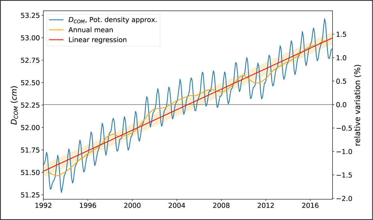
Figure A.1
Time series of global DCOM computed using the potential density approximation (see Table 1). As in Figure 2, the linear regression line (red) is shown with an envelope representing ± the standard error (shaded orange), and the annual mean is superimposed (orange). Corresponding variations relative to the mean are indicated on the right axis.
Appendix B
Depth Anomaly for Simple Density Profiles
Consider a water column of depth H with stable potential density profile . Neglecting compressibility effects, the dynamic height can be approximated as . The depth anomaly then simplifies to,
For a linear stratification, the mean-N2 value is constant, where is the potential density difference between the bottom and the top of the water column, and
For a two-layer stratification, of depths H1 and , the depth anomaly is,
The depth anomaly reaches its maximum when the two layers have equal depth , with , and it tends toward zero if any of the two depths goes to zero. This shows how the vertical shape of the density profile influences the depth anomaly and provides a method to attribute an effective stratification depth. For example, a linear stratification has the same depth anomaly as a two-layer stratification with an upper layer depth .
It is easy to show that the maximum depth anomaly that a given water column can attain for a given is in fact reached in the two equal-depth layer case. Rewriting Equ. (B1) by separating contribution above and below the center of volume, we obtain,
Noting that the integrand is everywhere positive, the integral is maximized when the integrand is maximized everywhere, i.e., for any (QED).
Notes
Data Accessibility Statement
The ECCO data are publicly available at https://ecco-group.org/products.htm. The analysis presented in this manuscript was done partly using the ECCOv4-py software package (https://ecco-v4-python-tutorial.readthedocs.io) under the MIT License. Additional analysis is done using the xmitgcm package (https://github.com/MITgcm/xmitgcm) under the MIT License. The equation of state calculation was done using the gsw python package https://teos-10.org. Analysis scripts employed in this manuscript are publicly available at https://github.com/fabien-roquet/ECCO_centre_of_mass.
Acknowledgements
The computations were enabled by resources provided by the National Academic Infrastructure for Supercomputing in Sweden (NAISS), partially funded by the Swedish Research Council through grant agreement no. 2022-06725. This project is funded by the Swedish Research Council (VR project 2023-04600).