
1 Introduction
Data assimilation is widely practiced in the atmospheric and ocean sciences to improve estimates of the state of a given dynamical system, and possibly its parameters, by using observation information and characterizing uncertainties. Uncertainty in the state estimates is quantified through the estimation error covariance. The evolution, or propagation, of the estimation error covariance in time is an important component of modern data assimilation schemes.
Generally, covariance propagation is implied by the propagation of the state. In fact, the same discrete dynamical model that is used to propagate the state estimate, or possibly a linearized version of it, is typically used also to approximate the propagation of the covariance matrix. Kalman filters, for example, propagate the covariance matrix explicitly using the same discrete dynamical model defined for the state propagation (Jazwinski, 1970; Kalman, 1960). Variational-based schemes that evolve covariances, such as 4D-Var, evolve the covariance matrix implicitly through a tangent linear model and its adjoint during the minimization of the cost function (Jazwinski, 1970; Lorenc, 2003; Thépaut, Hoffman and Courtier, 1993). Ensemble-based methods, such as the ensemble Kalman filter (EnKF), approximate the evolution of the covariance matrix through the (generally nonlinear) evolution of the individual ensemble members (Evensen, 1994, 2009).
Recent work in chemical constituent data assimilation has observed that full-rank covariance propagation can be quite inaccurate when using the same discrete dynamical model defined for discrete state propagation (Gilpin, Matsuo and Cohn, 2022, 2025; Lyster et al., 2004; Ménard and Chang, 2000; Ménard et al., 2000; Ménard, Skachko and Pannekoucke, 2021; Pannekoucke et al., 2021). Propagated covariances suffer from spurious loss and gain of variance and from inaccurate correlations both near and away from zero separation. These inaccuracies in the covariances become particularly pronounced in regions where correlation length scales approach grid resolution (Gilpin, Matsuo and Cohn, 2022, 2025; Lyster et al., 2004; Ménard et al., 2000). This behavior observed during full-rank covariance propagation raises the question of whether ensemble-based covariance propagation might also suffer from the same inaccuracies. Since the introduction of the EnKF by Evensen (1994), the main focus of effort has traditionally been on understanding and mitigating sampling error, which is due to covariance matrices being estimated from a limited ensemble (e.g., Evensen, 2009; Hamill, Whitaker and Snyder, 2001; Houtekamer and Mitchell, 1998; Whitaker and Hamill, 2012). The covariance propagation itself, via the evolution of the ensemble members, as a source of error has largely been overlooked in the literature.
For states that satisfy the linear advection equation and related hyperbolic partial differential equations (PDEs), we find in this work that ensemble-based covariance propagation is severely inaccurate, particularly when correlation lengths become small. We demonstrate this through a series of numerical experiments and compare these results with previous work that has considered the full-rank, explicit covariance propagation of the Kalman filter (Gilpin, Matsuo and Cohn, 2022, 2025). We are able to explicitly quantify the errors in covariance propagation because the exact continuum covariance dynamics are known. The continuum covariance dynamics is governed by a deterministic PDE that can be explicitly formulated and solved in special cases, and has been studied extensively by Cohn (1993) and Gilpin, Matsuo and Cohn (2022).
In these numerical experiments, we find that the propagation of the mean state by the ensemble is accurate, while at the same time, the ensemble-based covariance propagation is remarkably inaccurate, much more so than expected from either sampling errors or typical numerical discretization errors. The errors in the ensemble covariances, which can be at least one order of magnitude larger than errors in the ensemble mean, are relatively constant with respect to ensemble size, but increase rapidly as correlation lengths decrease. The ensemble variances themselves do not resemble the exact variance, exhibiting both spurious loss and gain of variance in some cases, or severe variance loss in others, neither of which can be addressed by the usual techniques of variance inflation. The ensemble correlations, while exhibiting some spurious long-range correlations as ensemble sizes decrease, can in fact be severely inaccurate also near the covariance diagonal. Methods such as covariance localization (Hamill et al., 2009; Hamill, Whitaker and Snyder, 2001; Houtekamer and Mitchell, 2001) cannot help to rectify this issue. In fact, we find that the ensemble covariances approximate the covariances propagated explicitly at full rank rather well, converging to these covariances as ensemble size increases. However, neither the ensemble covariances nor the full-rank, propagated covariances are consistent with the exact, known continuum covariance solutions and do not approximate the exact covariances with acceptable accuracy.
The primary source of the inaccuracy in both ensemble-based and explicit, full-rank covariance propagation, is a fundamental discrepancy between the discrete dynamical model that is built from the continuum state dynamics and the behavior of the continuum covariance dynamics. While the state and covariance are related by definition, as shown in Cohn (1993) and Gilpin, Matsuo and Cohn (2022), the solutions to the continuum covariance PDE behave in ways that are not expected when considering the state dynamics alone. As a consequence, the discrete dynamical model, which encodes the state dynamics, is unable to capture the correct covariance dynamics when correlation lengths become small. This is observed in our numerical experiments, and is also supported by the analysis of the variance dynamics in Gilpin, Matsuo and Cohn (2025) and the correlation dynamics here in Appendix A.
Errors in covariance propagation are sometimes attributed to a notion of “model error,” often represented by a stochastic forcing term that is added to the state propagation, and consequently a model error covariance matrix added to the covariance propagation (Daley, 1991, Ch. 13.3; Dee, 1995). In the present work, the true dynamical system is given exactly by a PDE for the state and covariance so that we can isolate the errors caused by discrete propagation and ensemble size. In one set of experiments, we have a perfect model for the state, in which the discrete dynamical model for the state yields exact solutions for any grid resolution. We see in these experiments that errors in the corresponding covariances can still be significant even when using a perfect model for the state.
While our experiments do not consider the impact of assimilating observations, our findings suggest potential problems for the measurement update step of a data assimilation cycle. The accuracy of the analysis state and error estimates obtained from assimilating observations relies on the accuracy of these time propagated covariances (Daley, 1991, Ch. 4.9). Thus, errors during covariance propagation, which we illustrate here, can negatively impact the full data assimilation cycle.
Our intention with this work is to demonstrate through a series of simple numerical experiments a fundamental problem with covariance propagation in data assimilation for advective dynamics: accurate state propagation does not imply accurate covariance propagation when using the same discrete dynamical model for each. Ensemble-based covariance propagation is popular because it is computationally tractable in these algorithms. As seen in our experiments, however, the impact of using the same discrete dynamical model on the covariances themselves has been overlooked in the literature and can be quite problematic. The goal of this work is thus to clearly present the problem and open the door to potential solutions.
This paper is organized as follows. We begin in Section 2 by reviewing the propagation of the discretized mean state and covariance in data assimilation algorithms, specifically for full-rank propagation of the Kalman filter and its ensemble approximations, such as for the EnKF. This is followed by the continuum formulation and a series of numerical experiments in Section 3. In these experiments, we compare the mean state and covariance estimated from the propagated ensemble with the exact mean state and covariance to illustrate the severity of the errors incurred during discrete covariance propagation. We then discuss these results in Section 4 in the context of the continuum dynamics and analysis presented in Cohn (1993) and Gilpin, Matsuo and Cohn (2022; 2025). A summary of the main conclusions is given in Section 5. Appendix A provides our analysis of the correlation dynamics approximated by the numerical schemes and identifies the error terms that produce the behavior observed in the numerical experiments.
2 Discrete State and Covariance Propagation
A data assimilation cycle typically consists of two steps, performed either in sequence (as in a Kalman filter) or simultaneously (as in 4D-Var, for instance). The first is a time propagation step (forecast), which evolves the system (e.g., the mean state, covariance, ensemble of states) forward in time according to the given dynamics. The second is the measurement update step (analysis) that incorporates the observation information and uncertainty using Bayesian inference to produce an updated state estimate and corresponding uncertainty. The focus of this work is on the time propagation step alone.
Let represent the N-vector discretized state of a dynamical system at time tk. This state is evolved forward to time according to
where is an propagation (state transition) matrix that represents the discretized model dynamics. For simplicity, we assume the state dynamics are deterministic and linear, with no forcing, random or otherwise.
If the initial state is random with mean , then the mean state at time tk, , satisfies the same discrete propagation as the state, (1), since is deterministic,
Along with the mean state, we can define the covariance matrix at time tk, where the i,j-th entry of the covariance matrix is defined as
where denotes the expectation operator and denotes the i-th entry of the vector (and similarly for the index j). Given an initial covariance matrix , the propagation of the covariance matrix from time tk to then follows from (1) – (3),
where superscript T denotes the transpose. Equation (4) defines full-rank covariance propagation and is the time propagation of the covariance matrix in the standard Kalman filter (Kalman, 1960; Simon, 2006, Ch. 4 and references therein). The variance at time tk is defined as the diagonal of the covariance matrix ,
and the correlation matrix at time tk is the covariance matrix normalized by the square root of the variances (standard deviations),
We can compare the mean state and covariance propagation, (2) and (4) respectively, with that of ensemble-based schemes, such as the EnKF. Ensemble-based data assimilation schemes begin with an ensemble of initial states for sampled from a distribution with initial mean and initial covariance (such as a Gaussian distribution, for instance), and they evolve this ensemble forward in time according to the discrete state propagation defined in (1). At a time tk, the exact mean state and exact covariance are estimated by the ensemble mean and ensemble covariance using the standard empirical estimators,
The ensemble variance can either be defined as the diagonal of the sample covariance matrix or, equivalently, directly from the ensemble using the (unbiased) empirical estimator,
The ensemble correlation matrix can then be defined using (6) by replacing the exact covariance and variance with the ensemble estimates in (8) and (9), respectively.
Since the propagation of the individual ensemble members satisfies (1), it follows directly from (1)–(3) that the sample mean and sample covariance satisfy the same propagation equations as the mean state and covariance , respectively,
Thus, the evolution of the mean state and covariance are approximated through the evolution of the individual ensemble members. Since the number ne of ensemble members is typically much less than the dimension N of the state vector, the sample covariance is a low-rank approximation of the full-rank covariance . It can be shown under certain hypotheses that in the limit as the ensemble size ne approaches infinity, the approximated evolution of the mean state and covariance by the ensemble, (10) and (11), respectively, converge to the full-rank propagation for the mean state and covariance, (2) and (4), respectively (Evensen, 2009, p. 44; Furrer and Bengtsson, 2007, p. 231).
While full-rank covariance propagation (4) and ensemble-based approximations (11) both propagate the covariance, the means of propagation can be interpreted differently. Full-rank covariance propagation, as implemented in a Kalman filter, propagates the covariance matrix directly with its own, explicit evolution equation, in parallel with the evolution of the state. Ensemble-based methods, in contrast, do not evolve the covariance matrix explicitly per se, but rather do so indirectly through the propagation of the individual ensemble members. From this perspective, one may expect that ensemble-based schemes, which do not evolve the covariance matrix directly, may not suffer from the same errors observed in full-rank covariance propagation. In the numerical experiments, we find that for advective dynamics, ensemble-based covariance propagation does in fact suffer from these same problems.
3 Numerical Experiments
The goal of the numerical experiments is to illustrate the following: for a given discrete dynamical model, represented by the matrix , ensemble-based propagation of the mean state is accurate (up to the order of the numerical scheme), while the ensemble-based covariance propagation can be remarkably inaccurate, far beyond that expected from sampling errors alone. We show that the ensemble-based covariance propagation faithfully captures the behavior produced by full-rank propagation, but neither approximates the exact covariance dynamics well. For these experiments, we consider states that satisfy versions of the advection equation for which the exact covariance dynamics are known. Thus, we can explicitly quantify the errors in both the ensemble-based and full-rank propagation schemes.
We start by defining the dynamical model for the state dynamics, then introduce the continuum framework from which we derive the corresponding continuum covariance dynamics and related quantities. We then consider two specific dynamical systems for the state, define the numerical discretizations, and describe the ensemble initialization. This is followed by the results of the experiments.
3.1 Problem setup
Motivated by atmospheric data assimilation, we consider continuum states for , where denotes the unit circle, that satisfy the following generalized advection equation:
where the velocity and scalar are deterministic. For our experiments, we will fix two choices of b that define two different types of advective dynamics motivated by specific applications in atmospheric and chemical constituent data assimilation.
3.1.1 Continuum framework
For states that satisfy the generalized advection equation (12), the exact continuum covariance dynamics are also known. Therefore, we can leverage this information to evaluate and interpret the errors observed in full-rank and ensemble-based discrete covariance propagation. The full derivation and analysis of the continuum covariance dynamics are given in Cohn (1993) and Gilpin, Matsuo and Cohn (2022), and we summarize the important concepts here.
Analogous to the discrete case in (4), we can define the continuum covariance for spatial variables , associated with continuum states q,
where denotes the mean state for . Observing that the state dynamics are linear and coefficients v and b are deterministic, the continuum mean state satisfies the same PDE as q, (12). Following the definition of the covariance in (13), satisfies its own PDE,
where the subscripts 1,2 denote the quantities evaluated with respect to the spatial variables x1 and x2 (see Cohn, 1993; Gilpin, Matsuo and Cohn, 2022, for further details). We refer to this equation as the continuum covariance equation.
To make the connection between solutions to the continuum covariance equation (14) and the discrete, full-rank covariance propagation in (4), we first define the propagation of the continuum state q from time tk to time ,
The operator is the fundamental solution operator associated with (12) (Gilpin, Matsuo and Cohn, 2022, p. 891) defined on the space of square-integrable functions on the unit circle, , where means that the L2 norm of f is finite, ,
Discrete state propagation in (1) is therefore a discretization of (15).
Next, we define the covariance operator , defined on , whose kernel is given by (14),
With and its adjoint (see Gilpin, Matsuo and Cohn, 2022, Sec. 2.1), the evolution of the covariance operator from time tk to is given by
Full-rank, discrete covariance propagation defined in (4) is thus a discretization of (18).
For nonzero initial correlation lengths (see Gilpin, Matsuo and Cohn, 2022 and here in Section 4 for further details), we can define the continuum variance,
which satisfies its own PDE,
It then follows from the variance-correlation decomposition of the covariance,
that the continuum correlation satisfies
From the correlations, we can define a correlation length scale L(x,t),
where
This correlation length satisfies its own PDE (as derived in Cohn, 1993 and Gilpin, Matsuo and Cohn, 2025),
Observe that for a spatially varying velocity field (), the correlation length field will evolve over space and time, even if the initial correlation length is constant in space. In particular, satisfies the continuity equation, and therefore the average inverse correlation length is conserved in time,
This implies that regions of convergence in the velocity field (where ) will cause correlation lengths to shrink, and will be balanced by regions of divergence in the velocity field (where ) that will cause correlation lengths to grow. Thus, small correlation lengths are to be expected dynamically. We will see in the numerical experiments that these dynamics play a role during covariance propagation.
For these numerical experiments, we let the velocity v vary in space, but not in time,
In this case, we have exact solutions to all previously stated continuum equations (for the state, covariance, variance, correlation, and correlation length) given in Appen. B of Gilpin, Matsuo and Cohn (2022) and Appen. C of Gilpin, Matsuo and Cohn (2025).
3.1.2 Energy conservation
Motivated by chemical constituent data assimilation, we consider (12) with . These dynamics arise when q is the square root of a positive quantity that satisfies the continuity equation, such as concentration or density. In particular, we rewrite these dynamics into conservation form,
We refer to these dynamics as the energy conservation case, as the “energy” defined as , where is the L2 norm in (16), is conserved in time. The corresponding continuum covariance and variance equations satisfy conservation properties of their own, see Sec. 2 of Gilpin, Matsuo and Cohn (2025) for more details.
We discretize (28) using the Crank–Nicolson finite difference scheme, which applies a second-order centered-difference approximation of the spatial derivatives followed by the trapezoidal rule time-integration scheme (Crank and Nicolson, 1947). The propagation of the discrete state to time is defined as
where we assume periodic boundary conditions. Crank–Nicolson is a second-order (in space and time) accurate implicit scheme that is quadratically conservative when the velocity does not depend on time, as in our numerical experiments (27). Therefore, discrete versions of the continuum conservation properties of the state, variance, and covariance are preserved (see Sec. 2 of Gilpin, Matsuo and Cohn, 2025). Since the Crank–Nicolson finite difference scheme is an implicit scheme, we do not explicitly compute the propagation matrix and instead apply a linear solver to (29) at each time step. Similarly, the corresponding full-rank covariance propagation (4) is not implemented directly since we do not form explicitly. Instead, one time step corresponds to applying a linear solver twice, one application to compute , which applies (29) along the columns of , then , which applies (29) to the rows of .
The unit circle is discretized uniformly into grid points, . The time step is defined by the Courant number ,
where is the maximum value of the velocity field in (27). While the Crank–Nicolson scheme is stable for any value of , we take to define the time step . We run these experiments to a final time , which corresponds to slightly after a full time period for these dynamics.
3.1.3 Pure advection
In addition to the energy-conserving case, we consider the pure advection case where , which has been studied in the chemical constituent data assimilation literature (Lyster et al., 2004; Ménard and Chang, 2000; Ménard et al., 2000; Ménard, Skachko and Pannekoucke, 2021; Pannekoucke, 2021; Pannekoucke et al., 2016, 2021; Sabathier et al., 2023). To remain consistent with those studies, we apply a first-order upwind forward-Euler finite difference scheme to define the discrete state propagation,
This is equivalent to a first-order semi-Lagrangian discretization scheme with linear interpolation. It is an explicit scheme, therefore we form the propagation matrix explicitly to define the state propagation and mean state propagation in (1) and (2), and full-rank covariance propagation in (4). The spatial grid and time step are defined in the same way as for the energy conservation case. For a constant (in space) initial condition , this scheme is exact for any spatial grid, and therefore defines a perfect (discrete) model for the state propagation.
As noted in Gilpin, Matsuo and Cohn (2025), the upwind forward-Euler scheme has a transient phase in which numerical dissipation dominates before settling towards a roughly time-periodic behavior. Therefore, for the pure advection case, we run experiments to , slightly longer than the energy conservation case, so that solutions are no longer in the transient regime.
3.1.4 Ensemble initialization
The initial ensemble , is drawn from a multivariate Gaussian with constant initial mean state and initial covariance matrix . Initial covariances are constructed using the Gaspari–Cohn compactly supported approximation to a Gaussian (Gaspari and Cohn, 1999), their (4.10). These correlation functions depend on a single cut-off length parameter c that determines its region of compact support, i.e., where the correlations become identically zero. The cut-off length parameter c relates to the correlation length L(x,t) of (23) by
In our results, we use the initial value c to distinguish between the covariances in the various experiments. We take the initial variance to be one in all experiments; experiments with a spatially varying initial variance produced similar results to the unit variance case and are not shown. Initial ensemble members with negative values are discarded and replaced with new members that do not violate positivity. The Crank–Nicolson scheme (29) and upwind forward-Euler scheme (31) are not positivity preserving. We do not enforce positivity during propagation and allow for the relatively few instances where ensemble members become negative during propagation.
3.2 Results
In this section, we present the results from the numerical experiments and highlight important features. Interpretation of these results is then given in Section 4.
3.2.1 Mean state and variances
Figure 1 plots the average percent error in the ensemble mean (panels a and d), ensemble variance (panels b and e), and ensemble standard deviation (square root of the variance; panels c and f) relative to the exact mean state, exact variance, and exact standard deviation, respectively. These errors are plotted as a function of ensemble size and initial correlation length, denoted by the initial cut-off c in the legend. Errors are computed in the norm, which for an N-vector is defined as
The errors in the ensemble mean, variance, and standard deviation are then normalized by the norm of the exact mean state, variance, and standard deviation, therefore the results in Figure 1 are unitless and can be directly compared. Figure 1(a, b, c) corresponds to the energy conservation case, and Figure 1(d, e, f) corresponds to the pure advection case. In addition to the large ensemble , we calculate errors for ensemble sizes of . For each fixed ensemble size smaller than , we randomly draw from the ensemble of propagated states and compute the error in the mean state, variance, and standard deviation estimates. We repeat this 1000 times and average the error over these repetitions, which is plotted in Figure 1. For reference, we also include the percent errors in the mean state propagated directly by (2) and the percent errors in the covariance diagonals and the square root of the covariance diagonals approximated by (4).
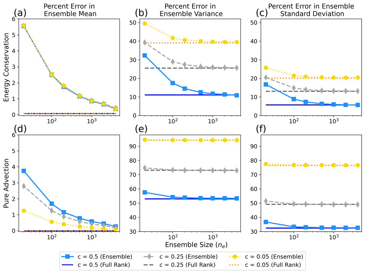
Figure 1
Percent error in the mean, variance, and standard deviation estimated from ensemble and full-rank propagation. Panels (a) and (d) plot the average percent error in the ensemble mean (scatter markers; Ensemble in the legend) and mean state from full-rank propagation (Full Rank in the legend) relative to the exact mean state. Panels (b) and (e) plot the average percent error in the ensemble variance (scatter markers; Ensemble in the legend) and covariance diagonals from full-rank propagation (Full Rank in the legend) relative to the exact variance. Panels (c) and (f) plot the average percent error in the ensemble standard deviation (scatter markers; Ensemble in the legend) and the square root of the covariance diagonals from full-rank propagation (Full Rank in the legend) relative to the exact standard deviation. All errors are plotted as a function of ensemble size (horizontal axis) and initial correlation length Lc (color; denoted by c in the legend). The top row (a, b, c) corresponds to the energy conservation case, and the bottom row (d, e, f) corresponds to the pure advection case. Errors are computed at the final time Tf for the two respective numerical experiments, see text for details.
The errors in the mean state estimated from the propagated ensemble, Figure 1(a, d), are as expected: the errors are small (a few percent) and decrease exponentially as the ensemble size increases. The errors in the ensemble mean converge toward the error in the mean state propagation in the full rank problem (2), where the percent error in the mean state for the energy conservation case is , and is exactly zero in the pure advection case since the upwind forward-Euler scheme propagates a constant mean state exactly. In the energy conservation case (panel a), the errors in the ensemble mean do not depend on the initial correlation length, which is expected due to the conservation properties preserved by the Crank–Nicolson scheme. In the pure advection case (panel d), there is some dependence on the initial correlation length. This is likely due to errors in the initial ensemble approximating the constant initial mean state , which then remains constant for all time (see Figure 2c, for example). In general, the errors in the ensemble mean are small and within what is expected for these methods.
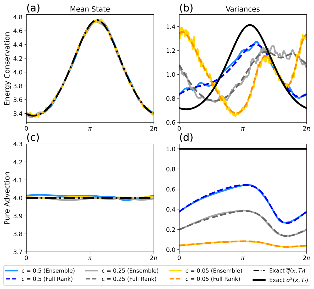
Figure 2
Comparison of exact mean state and variance with approximations by the propagated ensemble and corresponding full-rank propagation. Panels (a) and (c) compare the exact mean state (Exact in the legend) with the ensemble mean (solid color; Ensemble in the legend) and mean state propagated directly at full rank (dashed color; Full Rank in legend) for the different initial correlation lengths Lc (denoted by c in the legend) for the energy conservation (a) and pure advection (c) cases. The mean states propagated at full rank either identically or almost identically overlap with the exact mean state solution (black dashdot). Panels (b) and (d) compare the exact variance (Exact in the legend) with the ensemble variance (solid color; Ensemble in the legend) and variances approximated by full-rank covariance propagation (dashed color; Full Rank in legend) for different initial correlation lengths. The ensemble means and variances are calculated for ensemble size . Note the different vertical scales in each panel.
The behavior in the ensemble variance is in stark contrast to that of the ensemble mean, Figure 1(b, e). Across both cases, the errors in the ensemble variance are at least one order of magnitude larger than for the mean state, and they increase as the initial correlation length (proportional to c in the legend) decreases. Perhaps surprisingly, the errors in the ensemble variances are relatively constant with respect to ensemble size, particularly for the pure advection case. We can see in Figure 1(b, e) that the errors in the ensemble variances depend primarily on correlation lengths, which is consistent with what is observed during full-rank covariance propagation (Gilpin, Matsuo and Cohn, 2022, 2025). This means that sampling errors are not the dominant source of error in the ensemble variances. Sampling errors only contribute significantly for the smallest ensemble (20 members). Additionally, we see that the errors in the ensemble variance converge toward the errors in the covariance diagonals produced during full-rank covariance propagation. This indicates that the ensemble methods are approximating the solution to the discrete problem, namely (4), rather than solutions to the continuum covariance PDE.
A consequence of the inaccurate ensemble variances is the inaccurate ensemble standard deviations, Figure 1(c, f). The errors in the ensemble standard deviations behave similarly to those observed in the ensemble variances. Due to the similar behavior in the ensemble variances and standard deviations, we focus on the variances going forward.
To better understand the contrast between the mean state and variance errors in Figure 1, Figure 2 compares the exact mean state and variance with their ensemble approximations in the large ensemble case (), i.e., the mean and variance corresponding to the right-most points in Figure 1(a, b, d, e). For comparison, we also plot the mean state propagated at full rank according to (2) and variances approximated by the corresponding full-rank covariance propagation (the diagonals from (4)). Figure 2(a, b) corresponds to the energy conservation case, and Figure 2(c, d) to the pure advection case.
As expected from Figure 1, the ensemble means approximate the exact mean state rather well, as does the mean state propagated directly according to (2). The ensemble variances, however, are strikingly inaccurate. Figure 2(b, d) shows that the ensemble variances approximate the covariance diagonals extracted from full-rank covariance propagation very well, while neither is anywhere close to the exact variance dynamics. The variance approximations in the energy conservation case, Figure 2(c), exhibit both loss and gain of variance. In fact, due to the conservation properties of the Crank–Nicolson scheme, the amount of variance lost is exactly equal to the amount of variance gained since the total variance is conserved in time. Thus, standard variance inflation, where the full ensemble variance is artificially inflated by a factor greater than one, may help in regions of variance loss, but not in regions of variance gain. In contrast, the pure advection case exhibits significant variance loss that is problematic for the larger initial correlation lengths, and becomes dramatically worse as correlation lengths decrease, even with a perfect discrete dynamical model for the state. Inflation schemes have been developed to address this loss of variance for this particular set of dynamics and numerical scheme (Ménard, Skachko and Pannekoucke, 2021), though it is not likely to generalize to higher-order schemes or to different dynamics, such as in the energy conservation case (Gilpin, Matsuo and Cohn, 2025, Appen. A).
3.2.2 Correlations
To compare with the variances, Figure 3 plots the average percent errors in the ensemble correlations and the correlations from full-rank covariance propagation relative to the exact correlations for the energy conservation and pure advection cases. These average percent errors are computed in the same way as for the mean state and variances in Figure 1, replacing the norm with the Frobenius norm, which is defined for an matrix as
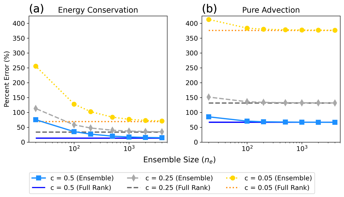
Figure 3
Percent error in the correlations estimated from the ensemble and full-rank propagation. Panels (a) and (b) plot the average percent error in the ensemble correlations (markers; Ensemble in the legend) and correlations from full-rank discrete covariance propagation (Full Rank in the legend) relative to the exact correlations as a function of ensemble size (horizontal axis) and initial correlation length Lc (color; denoted by c in the legend). Panel (a) corresponds to the energy conservation case and panel (b) corresponds to the pure advection case. Errors are computed at the final time Tf for the two respective numerical experiments and using the Frobenius norm.
The errors in the ensemble correlations are similar to those in the ensemble variances in Figure 1: errors depend primarily on the initial correlation length, increase as correlation lengths shrink, and converge to the errors from full-rank covariance propagation as ensemble size increases. Recall that the cut-off lengths c used to construct initial correlations define where these correlations become identically zero on the spatial grid (for the case, the one-dimensional correlations are nonzero on 67 grid points initially, and for , the one-dimensional correlations are nonzero on 33 grid points initially). We can also express the initial correlation length Lc of (32) in terms of the grid spacing , where
Thus, and . These initial correlations are reasonably well-resolved, and yet the errors in the ensemble correlations accumulated during the propagation are quite large. The case, which is the smallest initial correlation length considered ( and one-dimensional correlations are nonzero on seven grid points initially), has the largest errors. The case illustrates the severity of inaccurate discrete covariance propagation as covariances approach an uncorrelated/white noise regime for a fixed spatial grid. Increasing the spatial resolution, which one may suspect would help alleviate these errors, can be interpreted in this context as increasing the cut-off length (e.g., increasing to corresponds to increasing the spatial resolution by a factor of two). We see, however, that errors in the correlations persist, even when the correlations themselves are reasonably resolved.
Figure 3 reflects the global, cumulative errors in the correlations, and while Figure 3 allows us to distinguish between the errors due to propagation and the errors due to limited ensemble size (sampling error), as in Figure 2, these contributions become more clear when examining the correlations themselves. Figures 4 and 5 show selected one-dimensional correlations approximated from the large ensemble (), a small ensemble (), and correlations extracted from the corresponding full-rank covariance propagation. These are compared with the exact correlations for the energy conservation and pure advection cases, respectively.
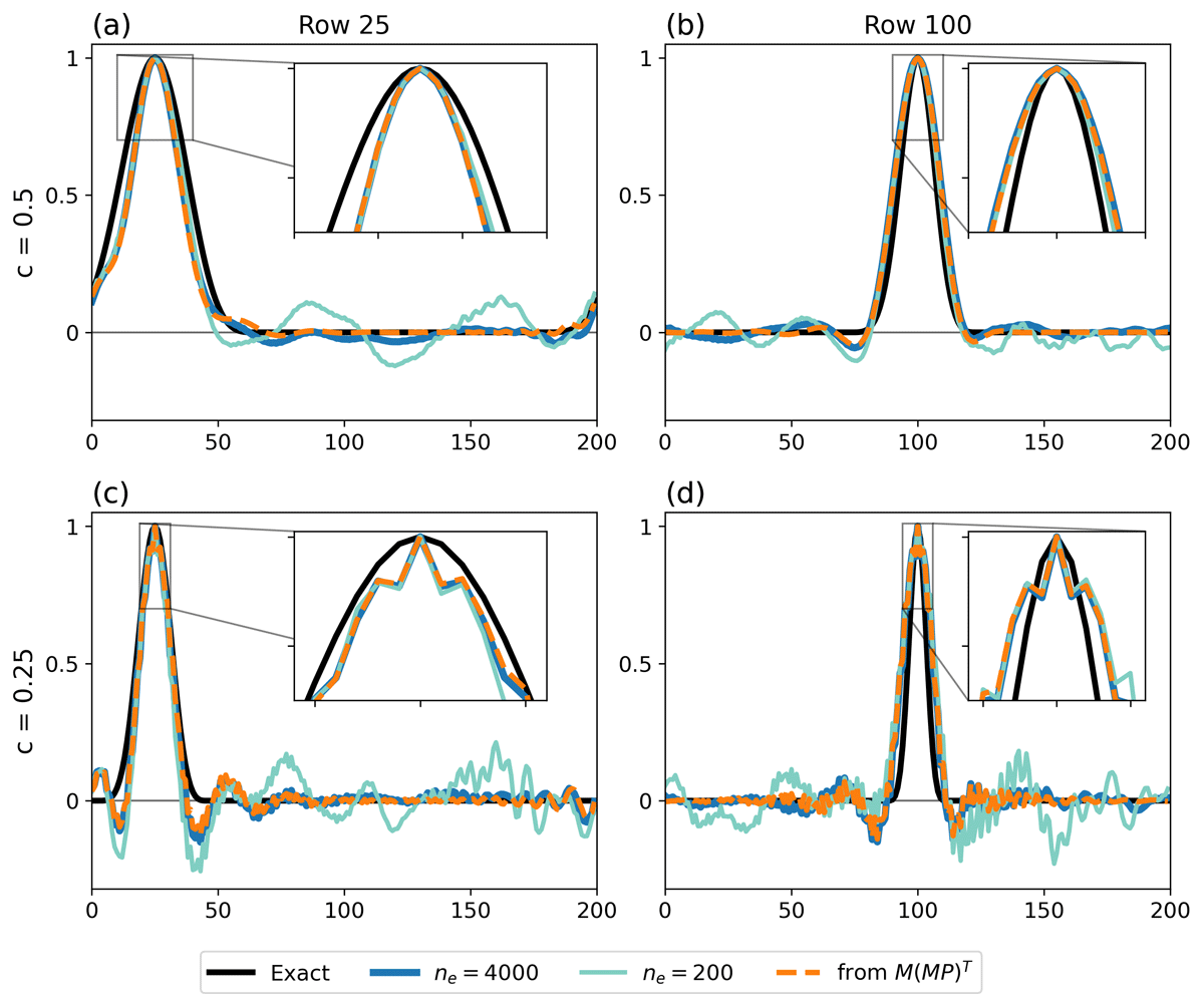
Figure 4
One-dimensional correlations for the energy conservation case. Each panel plots the exact correlation (solid black), correlation from full-rank covariance propagation (dashed orange), with ensemble correlations for (solid blue) and (solid light teal) at the final time for the energy conservation dynamics. Panels (a) and (b) correspond to an initial covariance with and (c) and (d) with . Row 25 of the correlation matrix is shown in (a) and (c); row 100 in (b) and (d). In each panel, the inset axis shows a zoomed-in portion of the correlations near zero separation.
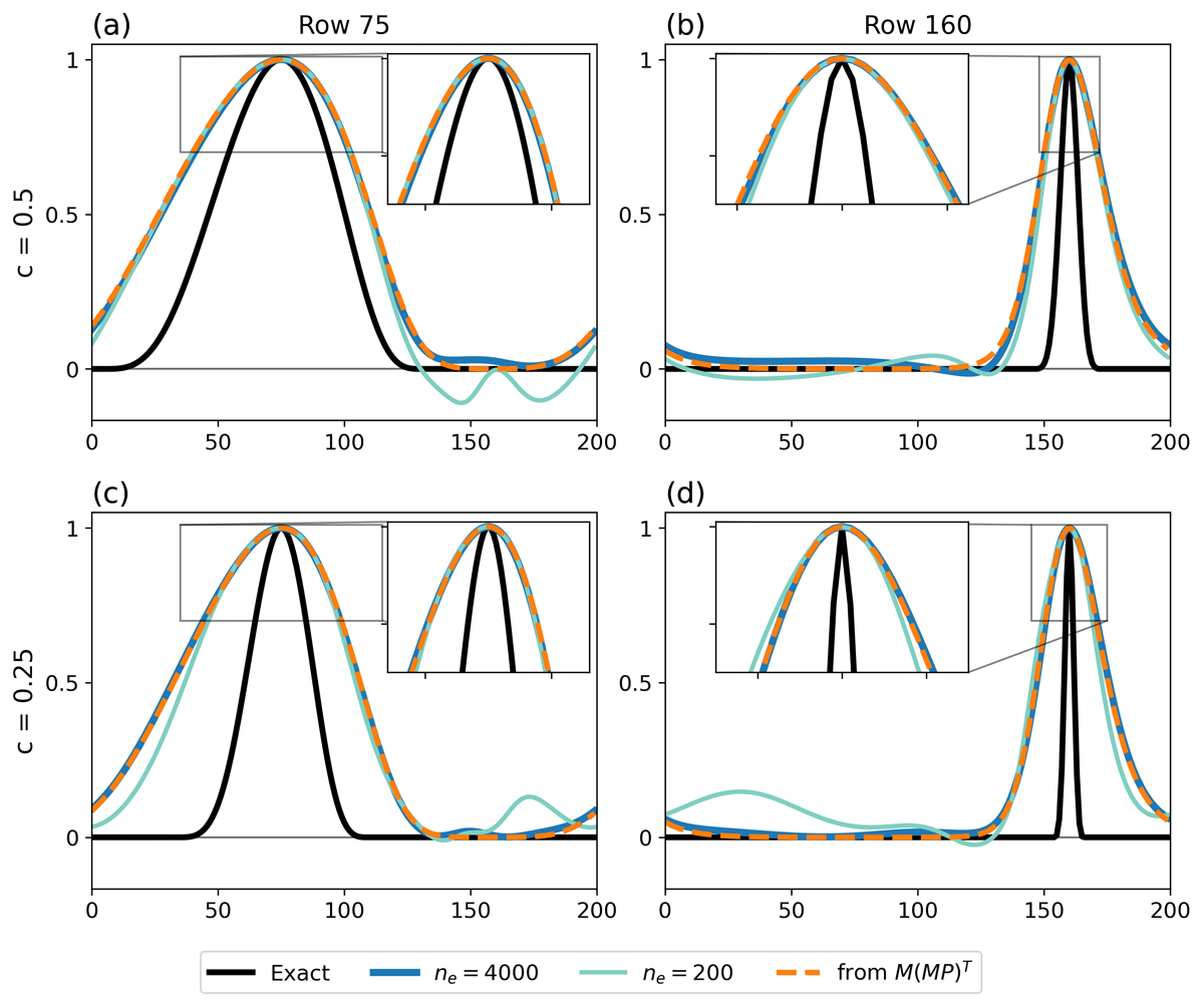
Figure 5
One-dimensional correlations for the pure advection case. Same as Figure 4 for the pure advection case, corresponding to and for row 75 in panels (a) and (c) and row 160 in (b) and (d).
For both state dynamics, we see similar behavior in the ensemble correlations as seen in the ensemble variances. The ensemble correlations approximate correlations extracted from full-rank covariance propagation rather well, while neither can successfully approximate the exact correlations. Near zero separation, the ensemble correlations and those from full-rank covariance propagation are nearly identical. The errors in these approximations depend on the dynamics and location within the correlation matrix. In the energy conservation case, Figure 4, correlations are under-approximated in some regions, and over-approximated in other regions. The oscillatory behavior in the energy conservation case is due to numerical dispersion and is expected from the Crank–Nicolson scheme (Beylkin and Keiser, 1997, p. 46).
The correlations in the upwind case, Figure 5, are quite inaccurate near zero separation, even more so than in the energy conservation case in Figure 4. Initially, correlation lengths for are twice as large as for , and both are fairly well resolved. Over time, the approximated correlations spread out dramatically and become almost indistinguishable between the and cases (compare down the columns of Figure 5). This lengthening of the correlations is related to the variance loss observed in Figures 1(e) and 2(d); this will be discussed further in Section 4.
Away from zero separation, spurious correlations in Figures 4 and 5 begin to appear in the small ensemble case, which are not present in the large ensemble or full-rank approximations. These spurious correlations are also reflected in the percent errors in Figure 3, but are not the primary source of error. Spurious, long-range correlations are to be expected as ensemble sizes decrease, particularly when estimating small (in magnitude) correlations. Covariance localization, which tapers long-range correlations, is often applied in ensemble-based schemes to address this issue (Hamill et al., 2009; Hamill, Whitaker and Snyder, 2001; Houtekamer and Mitchell, 2001). While covariance localization can mitigate spurious, long-range correlations due to sampling error, it cannot address the errors in the correlations near zero separation.
4 Discussion
The numerical experiments in Section 3.2 demonstrate the following:
The propagation of the mean state from the ensemble is accurate, while the variances and correlations approximated by the same ensemble are remarkably inaccurate.
Ensemble-based covariance propagation is a good approximation of full-rank discrete covariance propagation, yet neither can approximate the exact continuum covariance dynamics.
To understand why the covariances are so inaccurate in these numerical experiments requires taking a step back to understand the fundamental continuum aspects of covariance propagation.
On the surface, it may seem that the evolution of the covariance in ensemble-based covariance propagation and full-rank discrete covariance propagation are fundamentally different. However, the two methods are linked together by (1) the same discrete dynamical model , and (2) the underlying continuum covariance dynamics given in (14). Since the ensemble-based and full-rank covariance propagation produce nearly identical results, as we have seen, we can interpret the experimental results in Section 3.2 by studying the relationship between discrete covariance propagation, (4), and the continuum covariance dynamics, (14).
At an intuitive level, regions where correlation lengths become small correspond to regions with sharp gradients in the state, for example, in regions of strong wind shear (Lyster et al., 2004; Ménard et al., 2000). As a consequence, one may expect the numerical schemes (i.e., those used to build ) to struggle with discrete covariance propagation, as the accuracy of these methods begins to break down.
Regions with sharp gradients, or equivalently short correlation lengths, are particularly problematic for advective dynamics (12) when the initial state is random and gives rise to the continuum covariance equation in (14). As discussed in Gilpin, Matsuo and Cohn (2022), the hyperbolicity and the symmetry of the spatial derivatives in the continuum covariance equation (14) result in a peculiar behavior in the covariance dynamics that depends on the structure of the initial covariance, . This peculiar behavior is that the continuum covariance equation has two distinct types of solutions. First, when P0 has nonzero initial correlation lengths, the covariance solution has nonzero correlation lengths for all time (i.e., remains spatially correlated), and the dynamics along satisfies the variance equation (20). Second, if the initial covariance P0 is spatially uncorrelated (i.e., strictly diagonal), the covariance P remains spatially uncorrelated (diagonal) for all time, and the dynamics along satisfies instead what is called the continuous spectrum equation,
where we refer to as the continuous spectrum solution (Sec. 2.3 of Gilpin, Matsuo and Cohn, 2022). Equivalently stated, white noise remains white. These two solutions to the continuum covariance equation (14) are distinct when . Formally, this means there exists a discontinuity in the continuum covariance equation (14) in the limit as correlation lengths tend to zero.
While the initial covariance P0 may not be truly uncorrelated in practice, the continuous spectrum solution makes its presence known during discrete covariance propagation (4) when correlation lengths become small. This behavior manifests in error terms which arise in the continuum covariance dynamics that (4) is approximating. The analysis of the continuum dynamics approximated by (4) is broken down into the behavior along the covariance diagonal presented in Gilpin, Matsuo and Cohn (2025) and the behavior in the correlations presented here in Appendix A. The error terms in the approximated variance and correlation dynamics depend explicitly on powers of the ratio of the grid spacing and correlation length L(x,t), the same correlation length which satisfies (25) (see (45) and (49) of Gilpin, Matsuo and Cohn (2025) for the variances and (58) and (49) in Appendix A for the correlations). In fact, the form of the error terms in the approximated variance and correlation dynamics is nearly the same and in some cases mirrors each other in their behavior. These error terms are different from the typical discretization errors expected for a numerical scheme (i.e., local truncation error, LeVeque, 1992, pp. 104–105) and are a direct consequence of (4) approximating across the diagonal . Specifically, the inherent structure of (4) approximates across the discontinuity in the continuum covariance dynamics that distinguishes between the two solutions (see Gilpin, Matsuo and Cohn, 2025, for further discussion).
These error terms, depending on powers of the ratio that appear in the variance and correlation dynamics approximated by (4), explain the inaccurate behavior observed in the numerical experiments in Section 3.2. As correlation lengths shrink according to (25), for a fixed grid resolution, these error terms can become large enough to completely alter the approximated dynamics. In the energy conservation case, the leading error term appears in front of the advective, spatial derivative term, is of the form (see Gilpin, Matsuo and Cohn, 2025, their (45) for the variances; (58) in Appendix A for the correlations). We can compute the magnitude of this instantaneous error term at the start of propagation with the exact, initial correlation lengths Lc (35) for each of the three cases: for , ; , ; , . For and , these error terms start out small, but as correlation lengths shrink over time, these errors grow. As the correlation length L(x,t) approaches grid scale , the error term , a instantaneous error. These errors then spread through the covariance as it propagates and accumulate to produce the large percent errors in Figures 1 and 3, the loss and gain of variance seen in Figure 2(b), and corresponding errors in the correlations of Figure 4. The case has particularly large error at the start of the propagation that only becomes worse over time, resulting in the strikingly large errors in the variances and correlations compared to the and cases. We refer the reader to Gilpin, Matsuo and Cohn (2025) for a more detailed discussion on this accumulation of errors.
In the pure advection case, the first-order upwind spatial discretization yields a leading order error term of the form (see Gilpin, Matsuo and Cohn, 2025, their (49) for the variances; (49) in Appendix A for the correlations). In the approximated variance dynamics, this error term can be interpreted as a zeroth-order (with respect to derivative) dissipative term in the variance approximations, causing significant variance loss. The consequence is a relatively large dissipative term that immediately impacts covariance propagation from the start, causing the dramatic variance loss that propagates and accumulates over time. A corresponding error term of opposite sign occurs in the approximated correlation dynamics, mirroring the effect on the variances (namely, as variance is lost), as this loss is compensated by an increase in correlations. This relationship between variance loss and increased correlations has been observed (Ménard et al., 2000), and is now clarified by identifying these error terms explicitly. As noted in Gilpin, Matsuo and Cohn (2025) and Appendix A, the second-order error term that appears in the second-order centered differencing also appears in the first-order upwind case. This verifies that the underlying problem with discrete covariance propagation is not dependent on the discretization scheme or particular form of the advection equation (12). However, the impact of the error term on the upwind case is less, as this zeroth-order dissipative term is -times larger in magnitude.
While the initial correlation length scales in these numerical experiments are reasonably resolved, it is the shrinking correlation lengths over space and time that drive the inaccurate discrete covariance propagation. For the advective dynamics in (12), correlation length scales will shrink and grow according to (25). In general, regions of wind shear, i.e., sharp gradients in the velocity field, will continually produce smaller correlation lengths, cascading into smaller scales (Lyster et al., 2004, pp. 2327–2328). In the context of a full data assimilation cycle, assimilating uncorrelated observations generally shrinks correlation lengths in the analysis state estimate (Ménard, Skachko and Pannekoucke, 2021). This shrinking of correlation lengths during the measurement update will amplify the error terms in the approximated variance and correlation dynamics, producing errors that will be carried into the proceeding time propagation step. As correlation lengths continue to shrink, either dynamically or during the measurement update, a finer grid resolution (smaller ) will be necessary to ensure these error terms produced by (4) remain small. When taking into account the computational cost of decreasing , even in modest-sized systems, increasing spatial resolution may not lead to a simple fix for the variance and correlations.
To see that ensemble-based covariance propagation is almost identical to full-rank covariance propagation is both surprising and not surprising. One would expect that as the number of ensemble members ne becomes large, the ensemble covariances should approximate the covariances propagated at full rank by (4). This is verified in our numerical experiments. What is perhaps surprising is that the propagation of the mean state by the ensemble is accurate while the ensemble covariance is not, all while using the same discrete dynamical model defined by the state dynamics. These simple numerical experiments, together with previous analysis, bring to light a potentially fundamental problem for data assimilation with states that satisfy advective dynamics. The numerical experiments demonstrate that one cannot assume the propagation of the covariance, whether directly by (4), or indirectly by an ensemble, will be taken care of by appropriately propagating the state. While the continuum state and covariance dynamics are related, their behavior as PDEs is quite different and should therefore be treated as such. Covariance propagation schemes, as they currently stand, are not suited for covariance propagation for advective dynamics, and new methods should be explored with this behavior in mind.
While we do not directly consider the impacts of inaccurate covariance propagation at the measurement update step of a data assimilation cycle, these results shed light on potential problems that can arise during the assimilation of observations. Analysis state estimates of a data assimilation filter implicitly assume that both the propagated (forecasted) covariance matrix and observation error covariance are accurate. It is often the case that either one or both of these covariance matrices are not accurate in some way, resulting in analysis errors that typically underestimate the true analysis error (Daley, 1991, pp. 143–148). We observe in our numerical experiments that the propagated covariances can be quite inaccurate compared to the mean state, therefore these errors will be carried through to the measurement update to produce inaccurate analysis state estimates and errors.
5 Conclusions
We conclude with a summary of the key findings from this work. Through a series of simple numerical experiments, we have demonstrated that accurate mean state propagation by an ensemble does not imply accurate covariance propagation when correlation lengths become small. For states that satisfy the linear advection equation and its variants, the exact continuum covariance dynamics are known, and we have compared the mean state and covariance estimated from a propagated ensemble of states with the exact mean state and covariance. From these experiments, we observe the following:
While the mean state estimates are accurate, the same cannot be said of the ensemble covariances. The errors in the ensemble variances and correlations are at least an order of magnitude larger than for the mean state and depend on the initial correlation length, rather than ensemble size, increasing as initial correlation lengths shrink.
The ensemble covariances converge to the covariances approximated by full-rank discrete covariance propagation, and neither approximates the exact continuum covariance well.
The primary source of error in ensemble-based covariance propagation is due to the discrete covariance propagation itself, much more so than typical sampling errors due to finite ensemble size.
In particular, these numerical experiments demonstrate that ensemble-based covariance propagation produces covariances that are nearly identical to those produced during full-rank, discrete covariance propagation. This implies that while each propagation scheme may seem different, the underlying problem is what connects the two, namely the discrete dynamical model and the continuum covariance dynamics (14). The analysis of the errors in full-rank covariance propagation in Gilpin, Matsuo and Cohn (2025) for the variances and for the correlations here in Appendix A identifies the error terms that produce the inaccurate discrete covariance dynamics. These terms involve powers of the ratio of the grid resolution and the correlation length L(x,t). We observe that these error terms can be problematic even for well-resolved correlations with modest correlation length scales. The resulting errors in both the full-rank and ensemble-based covariances are severe, and for the ensemble-based covariances in particular, cannot be rectified by the standard methods of inflation and localization schemes.
While these numerical experiments are simple, the results are profound and enlightening. Ensemble-based data assimilation is widely practiced in the data assimilation community. While the discrete mean state propagation is understood to be accurate, at least within the limitations of grid resolution, the corresponding discrete covariance propagation is also assumed to be accurate and can therefore be overlooked. These simple numerical experiments illustrate that accurate discrete covariance propagation is not necessarily the case. The root of the problem lies in an inconsistency between the continuum covariance dynamics and the discrete covariance propagation defined from the discrete state. This work indicates that covariance propagation for advective dynamics can be problematic across data assimilation schemes that evolve covariances, independent of the propagation scheme, and can potentially cause issues during the measurement update step. Thus, a shift in mindset regarding covariance propagation in data assimilation may be necessary. Such a shift is already starting to take form in methods such as local covariance evolution introduced in Cohn (1993) and Gilpin (2023) and the parametric Kalman filter (Pannekoucke and Arbogast, 2021; Pannekoucke et al., 2016; Perrot, Pannekoucke and Guidard, 2022).
Appendices
A Analysis of the Correlation Dynamics
Figures 3, 4, 5 present the results for the correlations approximated by the ensemble and from the full-rank covariance propagation in comparison to the exact correlations for the two numerical experiments. These experiments demonstrate that, in addition to the variances, the correlations are poor approximations of the exact correlations. In this appendix, we provide an error analysis of the discretized correlations approximated by (4) to identify the terms that cause the errors in these approximations. This analysis follows the same procedure in Gilpin, Matsuo and Cohn (2025), which derives the continuum dynamics being approximated by (4) along the covariance diagonal. Here, we do the same for the correlations.
Although the results presented in Figures 3, 4, 5 correspond to a full discretization (i.e., the discretization of the continuum state dynamics in both space and time), it is sufficient to study the semi-discretization, namely discretization only in space, while leaving time a continuous variable. For this analysis, we will assume that the correlation is four times continuously differentiable in both spatial arguments, and the velocity is at least four times continuously differentiable in its spatial argument.
Recall that correlation for satisfies (22). Observe from (22) that the correlation dynamics are independent of b in the state dynamics, and for (as is the case in our numerical experiments), for all .
We discretize the unit circle such that for , , and assume periodicity. Quantities evaluated on the spatial grid are denoted by
Given a spatial discretization for the continuum state dynamics, we can derive the corresponding semi-discretization for the correlations, i.e., the time evolution of the elements Cij. To obtain this semi-discretization, we start with the semi-discretization for the covariance Pij, then apply the following decomposition,
where Pii and Pjj denote the i-th and j-th diagonal entries of the covariance.
We consider two cases corresponding to the schemes used in the numerical experiments in Section 3.2 and the analysis of the covariance diagonals in Gilpin, Matsuo and Cohn (2025). First, we consider a first-order upwind spatial discretization applied to the generalized advection equation (12) for general b, noting that for pure advection is a special case of this analysis. Second, we consider a second-order centered difference discretization applied to the energy conservation dynamics in (28). To ease the derivations and notation, we present the analysis in the reverse order of the numerical experiments, starting with the upwind differencing followed by centered differencing.
A.1 First-order upwind differencing
The pure advection case in Section 3.1.3 is a special case of the generalized advection equation, (12). Therefore, we will consider the generalized advection equation for this analysis (noting that taking corresponds to pure advection). Consider (12) and apply a first-order upwind discretization to the spatial derivative qx to obtain the semi-discretization for the state,
To define the corresponding semi-discretization for the covariance, we first define the covariance Pij in terms of the error ,
The semi-discretization for the covariance then follows,
To derive the semi-discretization for the correlation, replace Pij in (41) with (38), expand the time derivative on the left-hand side, and isolate ,
From (41), we have expressions for and , which we can substitute into (42). After a bit of simplification, we arrive at the semi-discretization for the correlation for first-order upwind differencing,
Note that for initially, the cancelation in the bracketed terms implies that for all time. Observe also that while this semi-discretization is defined for the full correlation matrix, the second set of terms inside the square brackets are local terms that average across the covariance matrix diagonal. Even though these averaging terms are local, they impact the whole correlation matrix.
The goal now is to derive the continuum dynamics approximated by (43). To do so, we first introduce a new quantity through a change of variables , ,
then expand about , which yields,
where we assume that . Note that C2 is the same quantity defined in (24) (see e.g., Cohn, 1993, pp. 3136–3137). We can also define in the same way as C0 above. We use this change of variables to expand the pairs of local averaging terms inside the square brackets of (43). These terms are second-order centered approximations of the correlation on the half grid, specifically,
and similarly for index j. We also use this change of variables and P0 to simplify the square root quantities. Considering the first term in (43), expanding the numerator about xi yields
Making these substitutions and with a bit of rearranging,
We have replaced and with the correlation length using (23). By expanding these terms back to xi and xj, we have the continuum correlation dynamics approximated by first-order upwind differencing,
Here, is , involving higher-order spatial derivatives of the correlation in xi and xj. The term is and contains higher-order error terms in powers of .
The first two terms on the right-hand side of (49) yield the correct correlation dynamics, (22). The first and second set of bracketed terms on the right-hand side of order are the typical, first-order error terms expected from first-order upwind differencing. The third and fourth set of bracketed terms on the right-hand side of (49) arise from the local averaging terms in the square brackets of (43). These error terms depend on powers of the ratio and can become significant as correlation lengths become small for fixed .
The third set of bracketed terms on the right-hand side of (49) can be considered as a first-order error term that causes correlations to increase when C is positive, and to decrease when C is negative. In our numerical experiments, the initial correlation , and therefore by the correlation PDE (22), for all time. Since and by assumption, this term in our experiments is positive. Thus, correlations will grow over time, and faster for small correlation lengths. This error term is of the opposite sign and half the magnitude of an identical error term in the corresponding approximated dynamics along the covariance diagonal, Eq. (49) of Gilpin, Matsuo and Cohn (2025). The mirroring of this error term in the correlation and covariance diagonal yields two conclusions. First, this balancing of decreasing variance and increasing correlation is consistent with the conservation properties of the continuum correlation dynamics. Second, the primary source of error in the correlations is caused by (4) averaging across the covariance diagonal.
The fourth set of bracketed terms on the right-hand side of (49) is also a consequence of the local averaging terms in (48), though its impact on the correlation dynamics is generally less than the first-order error term that precedes it. This term is important when comparing these approximated dynamics with those from the centered differencing case discussed in the next section.
A.2 Second-order centered differencing
The Crank–Nicolson finite difference scheme in Section 3.1.2 applies a second-order centered difference spatial discretization to (28). Therefore, we proceed here in the same way, applying second-order centered differencing to the spatial derivatives and qx in (28) to define the semi-discretization for the state,
Following the same procedure outlined in the first-order upwind case, we arrive at the semi-discretization for the covariance,
and the corresponding semi-discretization for the correlation,
Observe that the semi-discretization in the centered difference case is quite similar to the upwind case. The second term in each of the square brackets is the same type of local averaging term seen in the upwind case that produces correlation quantities along the half grid. In addition, by pairing the first and second terms and the third and fourth terms together, these reflect flux-like spatial derivatives also on the half grid, noting that the velocity terms are grouped in such a way to make this averaging on the half grid more clear.
We derive the continuum dynamics approximated by (52) using the same procedure applied to the upwind case with a few additional terms. The pairs of local averaging terms within each of the four square brackets are expanded following (46) and
There are two sets of square root terms that need to be replaced, where one set can be replaced with (47), and the other with the following,
as in (47). In addition, the velocity terms represent (second-order) centered approximations of velocities along the half grid, which we see in the following expansions,
and similarly for index j. Making use of this expansion for the velocity and replacing the square root quantities in (52), we arrive at
In the last step, we expand terms back to xi and xj. We then obtain the continuum dynamics being approximated by the centered difference scheme,
The term is involving higher-order spatial derivatives of the correlation, velocity, and P0 in the xi and xj directions. The term is and contains higher-order terms involving powers of .
As observed in the upwind case, the first and second terms on the right-hand side of (58) recover the correct correlation dynamics of (22). The first, second, and third sets of terms in the square brackets are the typical, second-order error terms expected for the centered difference scheme. The fourth set of bracketed terms on the right-hand side of (58) is a direct consequence of the local averaging terms in (52), and like the upwind case, depends explicitly on the ratio of the grid resolution and correlation length L. Thus, as correlation lengths become small, these error terms become large and corrupt the correlation propagation by (4). Unlike the upwind case, where correlations grow over time, the sign of the fourth bracketed term on the right-hand side of (58) can change. This is reflected in Figure 4, where in the correlations from the ensemble and (4) are under-approximations in some regions and over-approximations in others.
A3 Concluding remarks
The correlation dynamics being approximated by (4) for the upwind and centered difference schemes in (49) and (58), respectively, clarify the errors observed in the numerical experiments, Figures 3, 4, 5. The errors in the correlations are caused by the local averaging terms in (43) and (52), which produce terms in the approximated correlation dynamics that depend on the ratio of the grid resolution and correlation length L. As correlation lengths become small for fixed , these error terms become large. In the upwind case, the term of order causes an increase in correlations for positive correlations, which mirrors the corresponding loss of variance along the diagonal. In the centered-difference case, the term of order results in over- or under-approximated correlations depending on the sign of the error terms.
The equations for the approximated correlation dynamics presented here are consistent with those derived for the covariance diagonal in Gilpin, Matsuo and Cohn (2025). Together, they provide a more complete picture of the inaccuracy of discrete covariance propagation for advective systems. The underlying problem is the disconnect between the inherent structure of (4) (i.e., the local averaging terms) and the peculiar behavior of the continuum covariance dynamics in (14) (its two types of solutions).
Data Accessibility Statement
The code used to run the numerical experiments and generate the figures in this article are available from the corresponding author upon request.
Acknowledgements
The author would like to acknowledge Dr. Stephen E. Cohn and Prof. Tomoko Matsuo for their time and expertise that helped to strengthen and clarify the contributions of this work. The author would also like to thank the three anonymous reviewers for their careful reading and thoughtful feedback that improved this work.
Competing Interests
The author has no competing interests to declare.
Author Contributions
The author contributed to the conceptualization, analysis, investigation, software development, visualization, writing, and funding acquisition.