
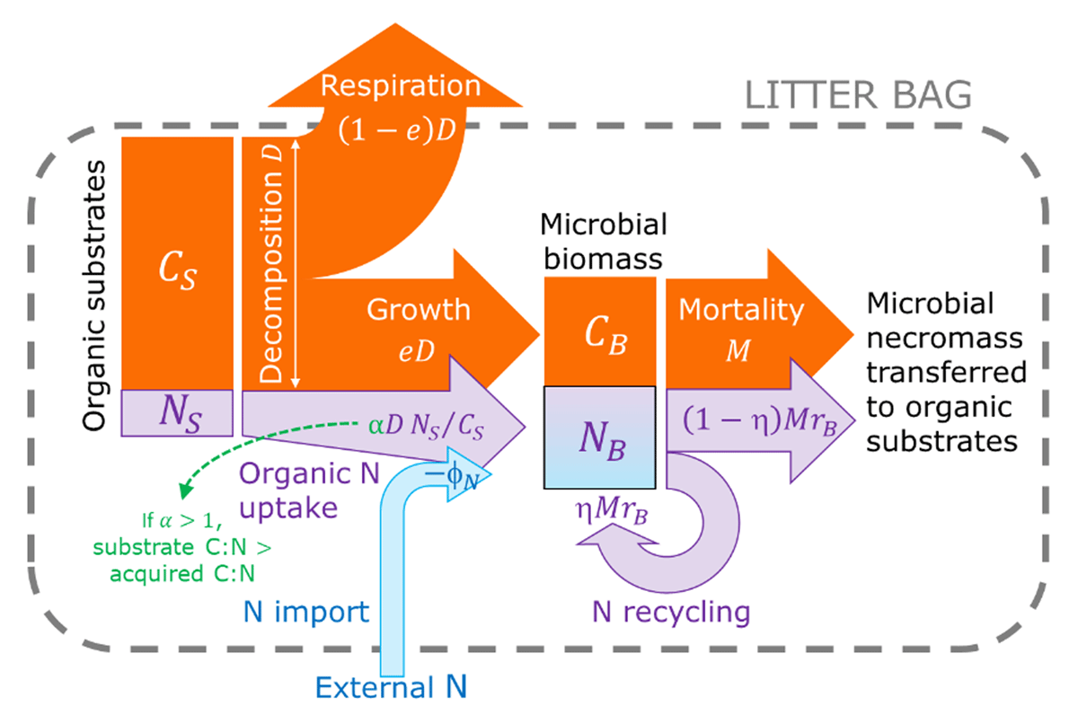
Figure 1
Schematic of the microbial biomass C and N exchanges [see symbol explanations in Table 1 and Eqs. (3) and (4)]. Orange, violet, and blue arrows indicate fluxes of organic C, organic N from residues, and inorganic or organic N from external sources, respectively. Necromass-derived organic substrates are returned to the substrate compartments (not shown for simplicity). The C:N ratio of acquired organic substrates can be lower than that of the original substrate if N is preferentially acquired (α > 1). The outer dashed box represents the modeled system (litter bag), which exchanges with the environment only through respiration and N release/import. In this illustration, N is imported (arrow pointing to NB) due to insufficient amount of substrate N—that is, external N accumulates within the litter bag).
Table 1
Symbol definitions and units (see also Figure 1). State variables are expressed in terms of C or N mass per litterbag.
| SYMBOL | EXPLANATION | UNITS |
|---|---|---|
| State variables and independent variables | ||
| cL | Fraction of initial litter C, cL = CL/CL,0 | – |
| CB | Microbial biomass C | g C |
| CL | Total litter C, CL = CS + CB | g C |
| CS | Litter substrate C | g C |
| nL | Fraction of initial litter N, nL = NL/NL,0 (nL > 1 when N is imported) | – |
| NB | Microbial biomass N | g N |
| NL | Total litter N, NL = NS + NB | g N |
| NS | Litter substrate N | g N |
| t | Time | Y |
| Rates and other calculated quantities | ||
| D | Litter decomposition rate | g C y–1 |
| G | Microbial growth rate, G = eD | g C y–1 |
| M | Microbial mortality rate | g C y–1 |
| φN | Net N import/release rate (net N import when φN < 0) | g N y–1 |
| ē | Mean C use efficiency throughout the decomposition process | – |
| Initial conditions | ||
| CL,0 | Initial total litter C | g C |
| C : NL,0 | Initial litter C:N ratio, C : NL,0 = 1/rL,0 | g C g N–1 |
| L0 | Initial lignin fraction | g lignin g litter–1 |
| NL,0 | Initial total litter N | g N |
| rL,0 | Initial litter N:C ratio, rL,0 = 1/C : NL,0 | g N g C–1 |
| Parameters | ||
| a | Exponent in Eqs. (15)–(17) | – |
| b | Half saturation constant in Eqs. (15)–(17) | g N g C–1 |
| b0 | Half saturation constant at zero lignin content in Eqs. (15)–(17) | g N g C–1 |
| b1 | Sensitivity to lignin content of the half saturation constant in Eqs. (15)–(17) | g N g litter g C–1 g lignin–1 |
| e | Microbial C-use efficiency (0 < e ≤ emax) | – |
| e0 | Microbial C-use efficiency when rL,0 = 0 (0 < e0 ≤ emax) | – |
| emax | Maximum microbial C-use efficiency (emax = 0.6) | – |
| rB | N:C ratio of microbial biomass | g N g C–1 |
| α | Preferential N acquisition coefficient (αmin ≤ α ≤ αmax) | – |
| α0 | Preferential N acquisition coefficient when rL,0 = 0 (αmin ≤ α0 ≤ αmax) | – |
| αmin, αmax | Lower and upper bounds for the fitting of the preferential N acquisition coefficient | – |
| η | N recycling efficiency (0 ≤ η < 1) | – |
| η0 | N recycling efficiency when rL,0 = 0 (0 ≤ η0 < 1 ) | – |
Table 2
Summary of model variants, including how C use and N recycling efficiencies are parameterized, which parameters are fitted to data, and which equations are used for the fitting.
| MODEL VARIANT | FIGURE LINE STYLE AND COLOR | PREFERENTIAL N ACQUISITION, α | C USE EFFICIENCY, e | N RECYCLING EFFICIENCY, η | FITTING PARAMETERS | FITTING EQUATION | |
|---|---|---|---|---|---|---|---|
| Time-invariant traits | Aflex | Dashed green | α | emax | 0 | α | Eq. (12) |
| Cflex | Dashed orange | 1 | e | 0 | e | Eq. (13) | |
| Nflex | Dashed blue | 1 | emax | η | η | Eq. (12) | |
| Dynamic traits | Adyn | Solid green | emax | 0 | α0 | Eq. (11) | |
| Cdyn | Solid orange | 1 | 0 | e0 | Eq. (11) | ||
| Ndyn | Solid blue | 1 | emax | η0 | Eq. (11) or Eqs. (13) and (14) |
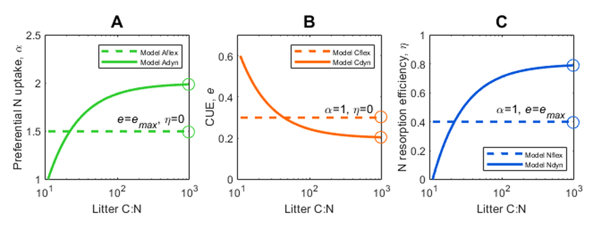
Figure 2
Relations between microbial traits and litter C:N during decomposition. (A) Coefficient indicating preferential N acquisition (α), (B) microbial C use efficiency (CUE, e), and (C) N recycling efficiency (η) as a function of litter C:N. Line styles refer to different model variants (legend); open symbols show the trait values that are estimated by fitting N import/release curves to the data. The equations for each of these relations are shown in Table 2.
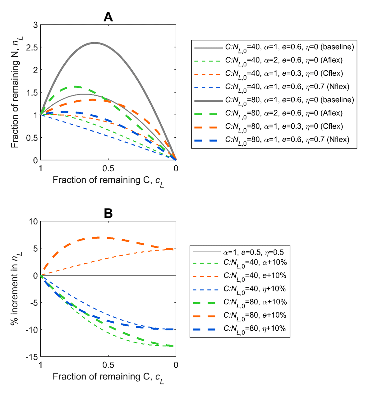
Figure 3
Effect of microbial traits on N import/release curves. (A) Fraction of initial litter N (nL) as a function of the fraction of initial litter C (cL), as predicted by models with time-invariant traits for different values of initial litter C:N ratio (C:NL,0 = 1/rL,0 in the model equations), preferential N acquisition (α), C-use efficiency (CUE, e), and N recycling efficiency (η). The gray curves are drawn assuming no preferential N acquisition, maximum CUE, and no N recycling, and serve as baselines to visualize the effect of flexible α, e, and η. (B) Sensitivity of nL to a 10% increase in α, e, and η from α = 1, e = 0.5, and η = 0.5, for different C:NL,0. In both panels, time progresses from left to right as cL decreases.
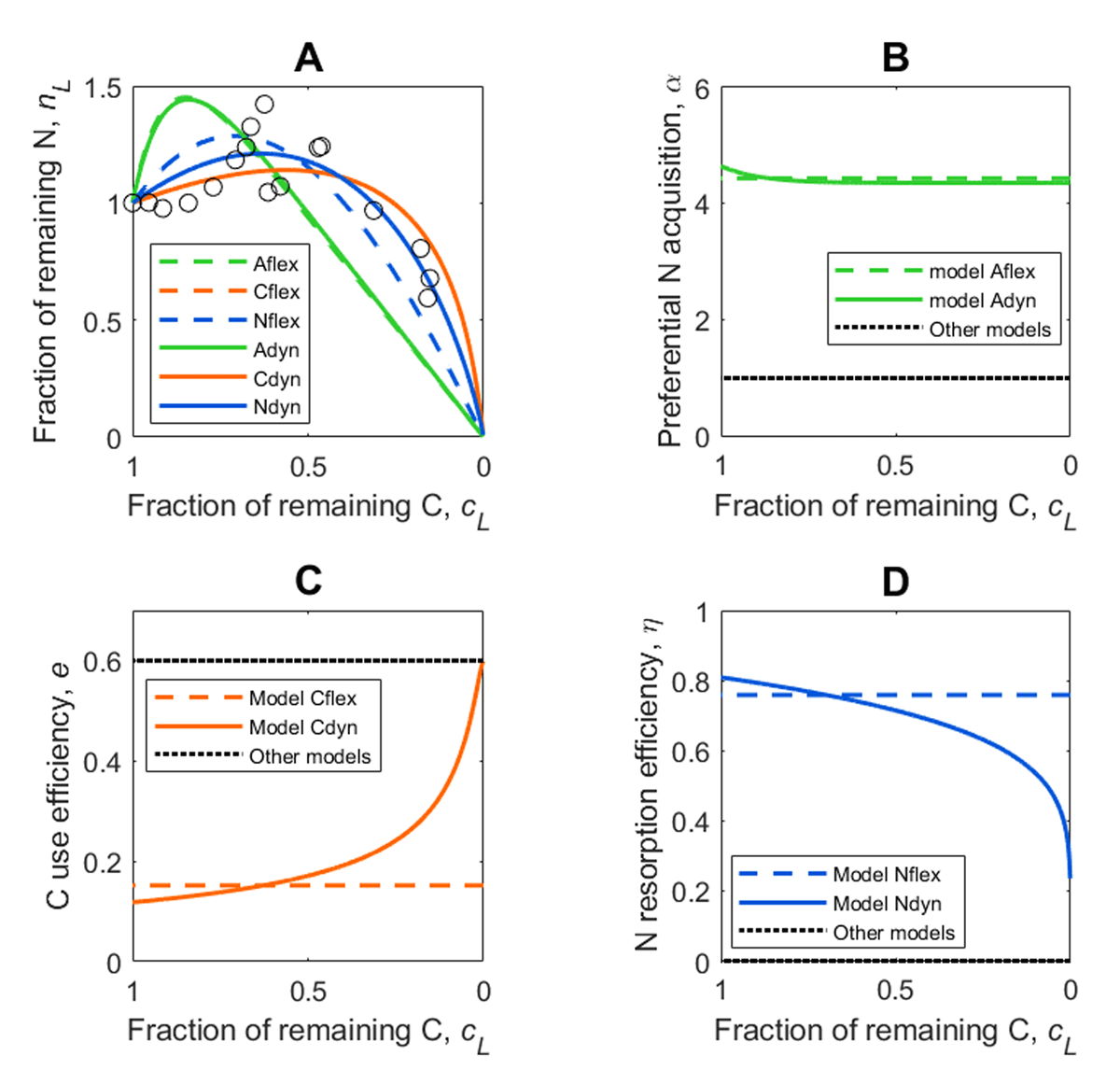
Figure 4
Example of N import/release data fitting with the six model variants (Table 2). (A) fraction of initial litter N (nL) modeled as a function of fraction of initial litter C (cL); (B) preferential N acquisition coefficient (α), (C) microbial C-use efficiency (e), and (D) N recycling efficiency (η) as a function of cL. Open circles indicate data for Pinus sylvestris from Melillo et al. (1989). In Figure 4A, the trajectories of models Cflex and Ndyn overlap so that the orange solid and dashed curves cannot be distinguished. In all panels, time progresses from left to right as cL decreases.
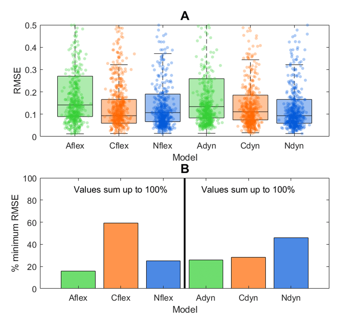
Figure 5
Comparison of model performances. (A) distributions of root mean square errors (RMSE) for the fractions of initial litter N (low values imply good fit) and (B) percentage of the datasets in which each model attains the minimum RMSE (among the different models assuming time-invariant traits (left of the vertical line) or dynamic traits (right of the vertical line). In Figure 5A, boxes show the median and quartiles, the whiskers indicate the extremes within 1.5 times the interquartile range, and dots are all RMSE values (not shown if higher than 0.5).
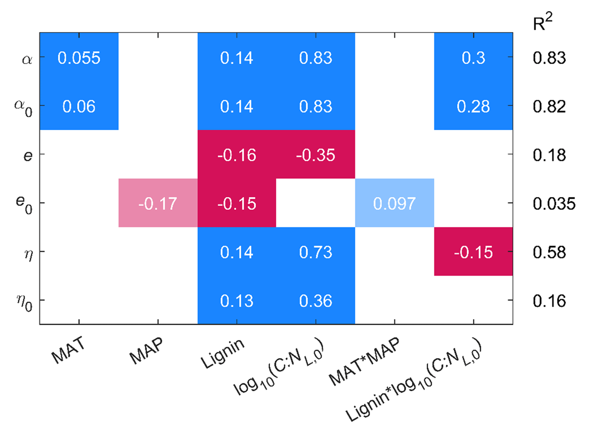
Figure 6
Chemical and climatic drivers of microbial traits. Results of linear models to predict microbial traits (preferential N acquisition α and α0, C use efficiency e and e0, and N recycling efficiency η and η0) as a function of mean annual temperature (MAT), mean annual precipitation (MAP), initial lignin content, initial litter C:N ratio (C:NL,0), and interactions between the two climatic factors and the two chemical characteristics. Each value represents a model coefficient (all variables are normalized), with colors indicating the direction of the effect (blue: positive, red: negative) and shading indicating the significance of the effect (dark colors: significant, p < 0.05; light colors: marginally significant, 0.05 < p <0.1; blank: not significant). On the right of the table the coefficients of determination (R2) for each model are reported.
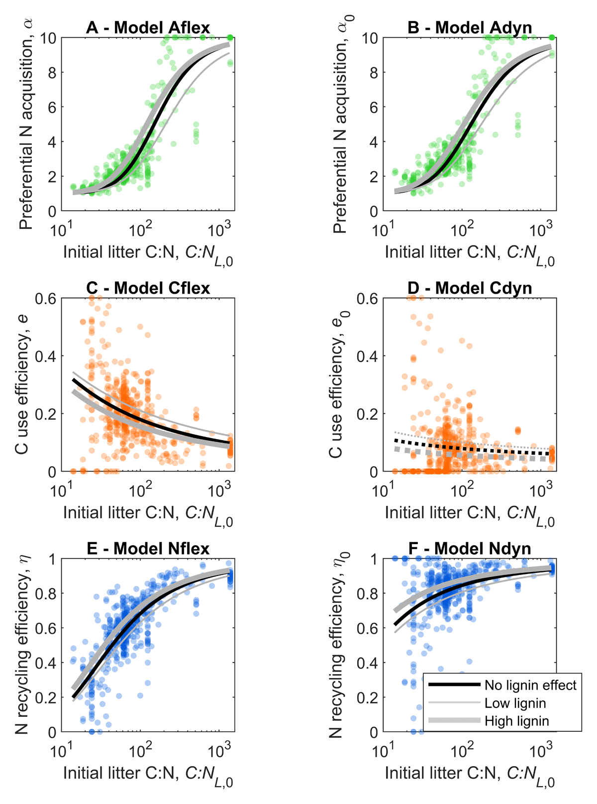
Figure 7
Litter chemistry effects on microbial traits. Model estimates of preferential N acquisition coefficient (α), C-use efficiency (CUE, e), N recycling efficiency (η) in the six model variants, as a function of the litter initial C:N ratio (C:NL,0): (A) α in model Aflex, (B) preferential N acquisition at zero litter N (α0) in model Adyn, (C) e in model Cflex, (D) CUE at zero litter N (e0) in model Cdyn, (E) η in model Nflex, (F) N recycling efficiency at zero litter N (η0) in model Ndyn. Curves are least square regressions of sigmoidal functions fitted to the estimated parameters [Eqs. (15)–(17); black: no lignin effects (full dataset), gray: including lignin effects (only data from sources reporting initial lignin content)]; dotted curves indicate that the trend when varying C:NL,0 is not significant (i.e., parameter a in the sigmoidal curve is not significantly different from zero). Gray curves are drawn at initial lignin contents corresponding to the 5th (labeled ‘Low’) and 95th percentiles (‘High’) of all lignin content data.
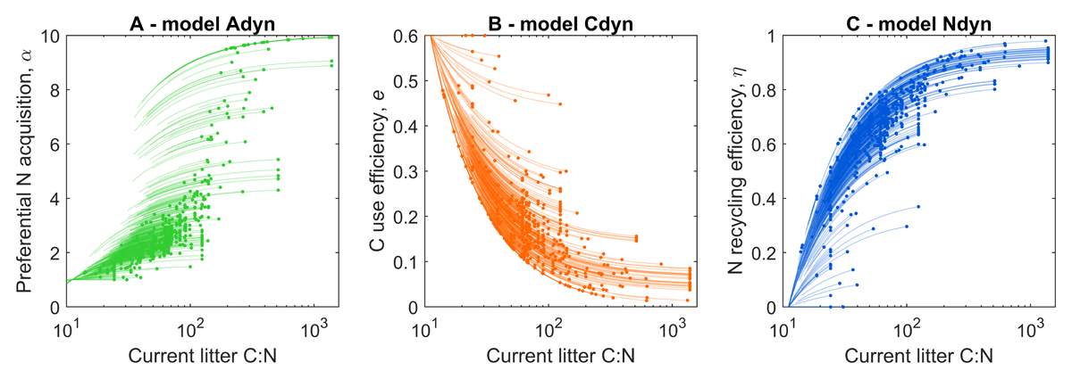
Figure 8
Temporal variations in microbial traits. Temporal changes in preferential N acquisition coefficient (α), C-use efficiency (e), and N recycling efficiency (η) in the three model variants that assume microbial traits can vary during decomposition, shown as a function of the current litter C:N ratio: (A) α in model Adyn, (B) e in model Cdyn, and (C) η in model Ndyn. Each curve represents a trajectory starting from the initial condition (indicated by a dot) and moving toward the left, as time progresses and litter C:N decreases.
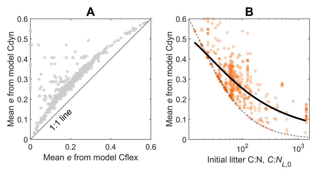
Figure 9
Mean C-use efficiencies. (A) comparisons of mean C-use efficiencies [ē from Eq. (20)] between models Cflex and Cdyn. (B) relation between ē and the initial litter C:N (C:NL,0) for model Cdyn. In Figure 9A, values of ē above the 1:1 line indicate that microbes convert more litter C into biomass than in model Cflex. In Figure 9B, the solid black curve is the least square regression of a sigmoidal function fitted to ē [Eq. (16); the trend when varying C:NL,0 is significant] and the thin dashed curve represents the limiting case of e0 = 0. Note that for all other model variants except Cdyn, ē = e or ē = emax, so relations between ē and C:NL,0 are the same already shown in Figure 7.