
Figure 1

Figure 2
Figure 3
Figure 4

Figure 5
Figure 6
Figure 7
Figure 8
Figure 9

Figure 10

Figure 11
Figure 12

Figure 13

Figure 14
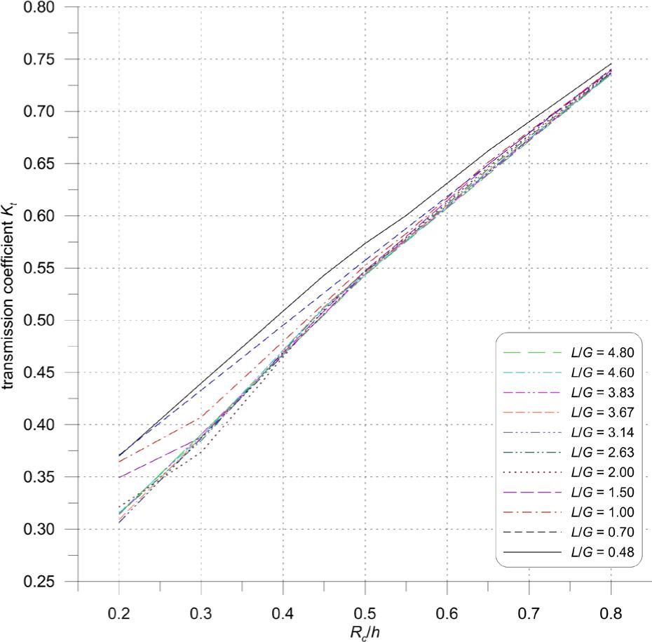
Figure 15
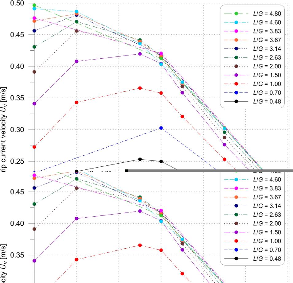
Figure 16
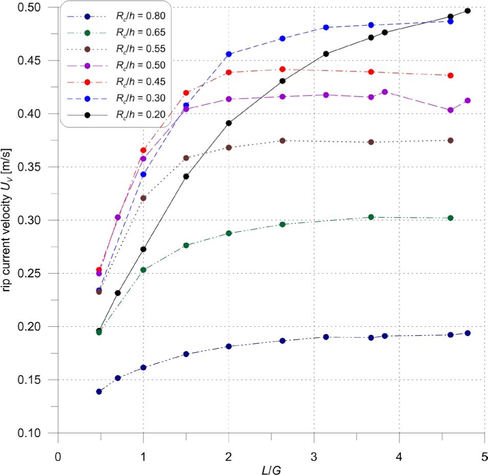
Figure 17

Coefficients (a and b) and goodness (R2) of linear approximation of the transmission coefficient Kt using the Rc/h ratio for various L/G values and for general approximation
| L/G | 0.48 | 0.70 | 1.00 | 1.50 | 2.00 | 2.63 | 3.14 | 3.67 | 3.83 | 4.60 | 4.80 | General |
|---|---|---|---|---|---|---|---|---|---|---|---|---|
| A | 0.627 | 0.616 | 0.644 | 0.675 | 0.717 | 0.712 | 0.717 | 0.715 | 0.704 | 0.706 | 0.702 | 0.686 |
| B | 0.253 | 0.248 | 0.227 | 0.205 | 0.178 | 0.180 | 0.171 | 0.178 | 0.180 | 0.183 | 0.180 | 0.198 |
| R2 | 0.997 | 1.000 | 0.997 | 0.995 | 0.994 | 0.995 | 0.996 | 0.995 | 0.997 | 0.996 | 0.998 | 0.987 |
Coefficients (A, B and C) and goodness (R2) of approximation (Eq_ 3) of rip current velocity UV using the L/G ratio for various Rc/h quantities
| Rc/h | 0.20 | 0.30 | 0.45 | 0.50 | 0.55 | 0.65 | 0.80 |
|---|---|---|---|---|---|---|---|
| A | 0.388 | 0.384 | 0.370 | 0.356 | 0.281 | 0.175 | 0.074 |
| B | 0.117 | 0.104 | 0.071 | 0.059 | 0.094 | 0.126 | 0.118 |
| C | 0.432 | 0.732 | 1.118 | 1.228 | 1.131 | 0.881 | 0.660 |
| R2 | 1.000 | 0.999 | 0.997 | 0.992 | 0.999 | 0.996 | 0.996 |