

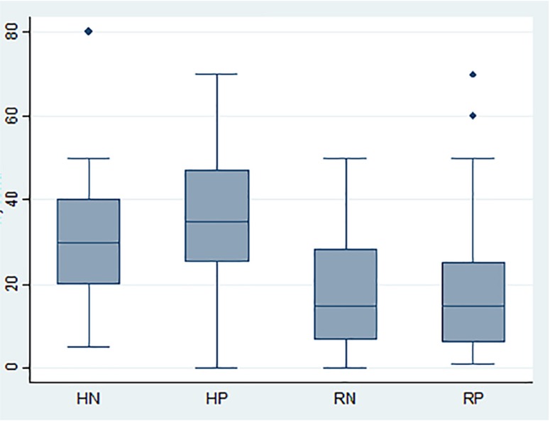
Fig. 1
Experiment: WTPs by treatment (in PLN). Notes: The blue rectangle represents the middle 50% of the data (from the first quartile to the third quartile), the line inside the box shows the median (the second quartile), and the whiskers represent the top and the bottom 25% values, excluding outliers, which are represented by dots.
Tab. 1
Descriptive statistics (monetary values in PLN)
| HypoN | HypoP | RealN | RealP | |
|---|---|---|---|---|
| n | 42 | 38 | 44 | 43 |
| Mean | 31.19 | 35.11 | 17.30 | 19.56 |
| Median | 30 | 35 | 15 | 15 |
| Standard deviation | 13.95 | 15.47 | 13.44 | 15.77 |
Tab. 2
Regression table: WTP values
| Ml b/z | M2 b/z | M3 b/z | M4 b/z | |
|---|---|---|---|---|
| hypothetical | 11.197*** (4.970) | 11.923*** (4.033) | 13.547*** (4.906) | 12.341*** (6.022) |
| framing_pos | 2.594 (1.189) | 3.320 (1.144) | 2.857 (1.033) | |
| information_e | 11.539*** (5.254) | 11.649*** (5.243) | 9.653*** (4.447) | 9.462*** (4.422) |
| needs_e | 2.423 (1.044) | 2.412 (1.036) | ||
| finance_e | 3.480 (1.411) | 3.463 (1.399) | ||
| using_mascara | 4.395 (1.283) | 4.299 (1.248) | ||
| price_30–50 | 6.167** (2.529) | 6.171** (2.523) | 5.792** (2.546) | 5.826** (2.569) |
| price>50 | 9.371*** (2.797) | 9.450*** (2.807) | 8.426*** (2.752) | 8.851*** (2.944) |
| cosm_expenses | 5.714** (2.309) | 5.662** (2.278) | 5.705** (2.431) | 5.569** (2.388) |
| the_same_masc | -3.358 (-1.401) | -3.469 (-1.432) | ||
| self_assessment | -2.304 (-0.941) | -2.242 (-0.911) | ||
| relationship | 4.397** (2.007) | 4.282* (1.931) | ||
| finaneial_syt | -0.793 (-0.359) | -0.871 (-0.391) | ||
| age | -1.083 (-0.869) | -1.080 (-0.863) | ||
| hypoXfram_pos | -1.650 (-0.381) | -2.481 (-0.608) | ||
| design_e | -5.826** (-2.390) | -5.902** (-2.434) | ||
| constant | 24.056 (0.924) | 23.760 (0.909) | 8.486*** (3.329) | 9.951*** (4.732) |
| N | 154 | 154 | 160 | 160 |
| R-sgr | 0.4604 | 0.4610 | 0.4401 | 0.4361 |
| F | 8.47 | 7.87 | 14.83 | 19.72 |
| Prok>F | 0.0000 | 0.0000 | 0.0000 | 0.0000 |
[i] * p<.10, ** p<.05, *** p<.01