

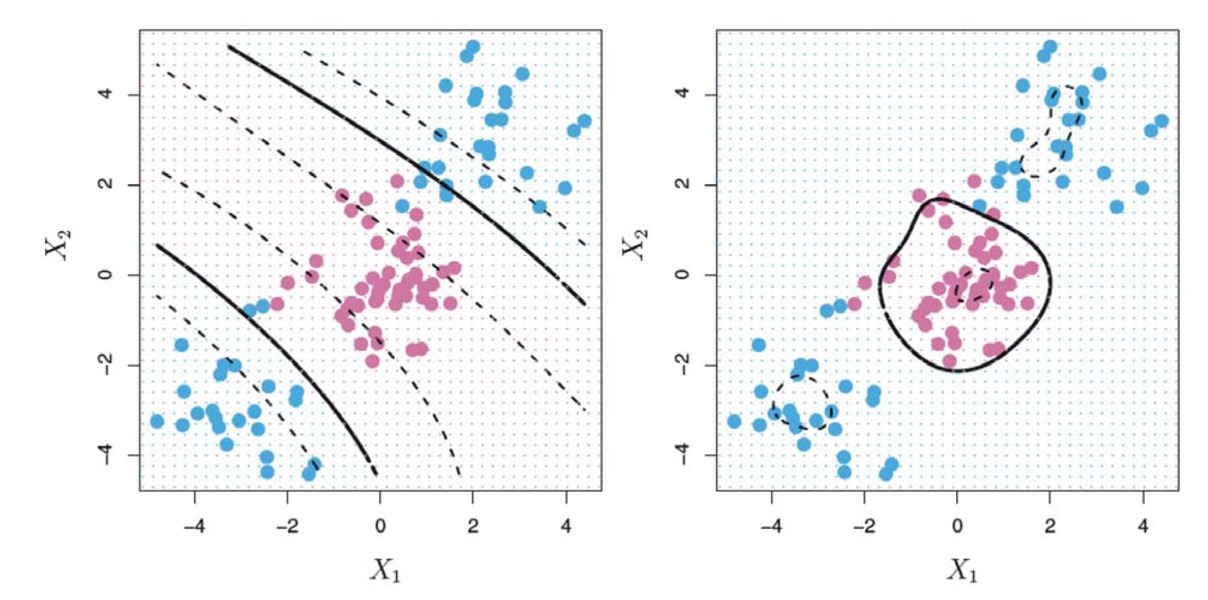
Fig. 2.1
Left panel: non-linear data divided by an SVM with a polynomial kernel of degree 3. Right panel: the same non-linear data divided by an SVM with a radial kernel
Source: James, G., Witten, D., Hastie, T., Tibshirani, R. An Introduction to Statistical Learning with Applications in R.
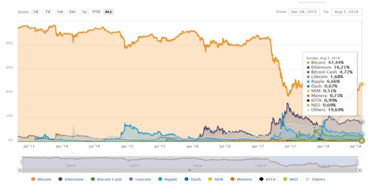
Fig. 3.1
Percentage of total market capitalization by dominance
Source: https://coinmarketcap.com/charts/
Note: the chart presents the dominance of the cryptocurrencies with the largest market capitalization over the period from 28/04/2013 to 05/08/2018.
Tab. 3.1
Descriptive statistics for 10 largest and 10 smallest cryptocurrencies by MarketCap in TOP100 as of date 01-08-2018
| The largest 10 cryptocurrencies in TOP100 as of 01-08-2018 | ||||||||
|---|---|---|---|---|---|---|---|---|
| Name | %ARC | %ASD | %MDD | IR1 | IR2 | Date of start | Volume, mUSD | MarketCap, USD |
| bitcoin | 118 | 75.8 | 69.7 | 1.6 | 2.6 | 01-10-2014 | 1888 | 43839225862 |
| ethereum | 437.7 | 145.2 | 84.3 | 3 | 15.7 | 20-08-2015 | 323 | 17124399552 |
| ripple | 226.7 | 164.6 | 87.1 | 1.4 | 3.6 | 01-10-2014 | 499 | 13468236361 |
| bitcoin-cash | 83.5 | 198.5 | 84.4 | 0.4 | 0.4 | 05-08-2017 | 699 | 6672807179 |
| eos | 516 | 253 | 87.9 | 2 | 12 | 14-07-2017 | 78 | 5220519698 |
| stellar | 228.6 | 178.8 | 82.6 | 1.3 | 3.5 | 01-10-2014 | 301 | 4634665748 |
| litecoin | 111.1 | 119.2 | 79.1 | 0.9 | 1.3 | 01-10-2014 | 80 | 3709789644 |
| cardano | 698.6 | 263.8 | 89.3 | 2.6 | 20.7 | 14-10-2017 | 32 | 2624893338 |
| iota | 48.4 | 188.4 | 82.9 | 0.3 | 0.1 | 26-06-2017 | 3059 | 2460207729 |
| tether | -5.4 | 45.7 | 49.9 | -0.1 | 0 | 15-03-2015 | 140 | 2233258238 |
| The smallest 10 cryptocurrencies in TOP100 as of 01-08-2018 | ||||||||
| Name | %ARC | %ASD | %MDD | IR1 | IR2 | Date of start | Volume, mUSD | MarketCap, USD |
| loom-network | 649.7 | 217.4 | 80 | 3 | 24.3 | 21-04-2018 | 2.8 | 98040413 |
| gas | 365.8 | 265.4 | 89.6 | 1.4 | 5.6 | 09-08-2017 | 2.6 | 91875052 |
| tenx | -97.6 | 247 | 99.2 | -0.4 | -0.4 | 10-07-2017 | 8.1 | 91154578 |
| nxt | 34.2 | 158.1 | 95.6 | 0.2 | 0.1 | 01-10-2014 | 2.8 | 90165499 |
| cybermiles | -44.8 | 202.2 | 87.4 | -0.2 | -0.1 | 04-05-2018 | 7.1 | 88375828 |
| nuls | 5083.5 | 382.2 | 79.1 | 13.3 | 854.8 | 22-03-2018 | 4.1 | 88067102 |
| byteball | 160 | 236.8 | 91.2 | 0.7 | 1.2 | 09-01-2017 | 0.56 | 86950232 |
| bibox-token | 53.2 | 265.7 | 87.9 | 0.2 | 0.1 | 08-06-2018 | 67.5 | 83456610 |
| odem | 89471 | 229.6 | 40.7 | 389.7 | 856638 | 01-08-2018 | 0.135 | 82906522 |
| electroneum | -92.5 | 243 | 95.3 | -0.4 | -0.4 | 15-11-2017 | 0.552 | 81946739 |
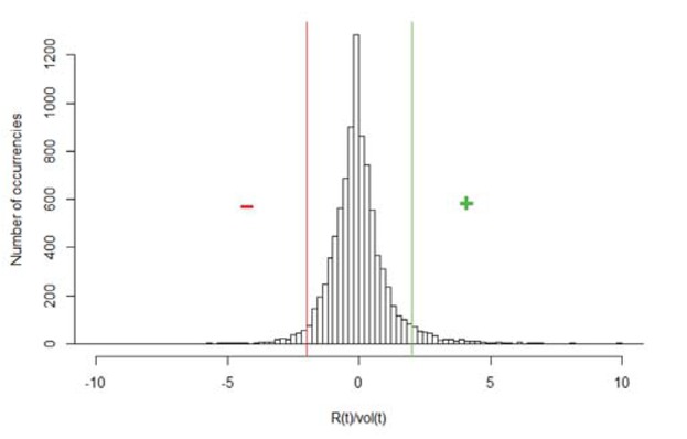
Fig. 3.2
Distribution of volatility-adjusted returns with 3-month history from 01/10/2014 to 12/31/2014 with cut-off lines to identify the number (training size) of the assets with the highest (green) and the lowest (red) volatility-adjusted returns to use for SVM training
Source: own work.
Note: the distribution of 91-days volatility-adjusted returns where the positive tail sets are the most positive volatility-adjusted returns, and the negative tail sets are the most negative. The vertical dotted lines represent the cut-off. The + and – regions are the ones used for SVM training.
Tab. 3.2
Technical indicators used for the creation of feature set to train SVMs
| Feature | Full name | Parameters |
|---|---|---|
| MOM, n days | Momentum for close prices, n days | n = 10 days |
| ΔV, n days | Volume change n days | n = 10 days |
| RSI | Relative Strength Index | n = 10 days |
| FI | Force Index | N/A |
| Williams %R | Williams Percent Range | n = 10 days |
| PSAR | Parabolic stop and reversal system | Acceleration factor by default set to 2% increasing by 2% with a maximum of 20% |
[i] Note: the table contains the list of six technical features used for running SVM and parameters set for calculations purposes.
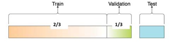
Fig. 3.3
Visualization of the data set splits and their proportions
Note: the figure represents in what proportion data is split to run the tuning of the meta parameters.
Tab. 4.1
Descriptive statistics of the SVM strategy compared with the benchmark strategies
| N | RE | %TC | V | %ARC | %ASD | %MDD | IR1 | IR2 | %MT | |
|---|---|---|---|---|---|---|---|---|---|---|
| S&P B&H | - | - | - | - | 13.6 | 15.5 | 14.2 | 0.9 | 0.8 | - |
| BTC B&H | - | - | - | - | 147.4 | 76.8 | 69.7 | 1.9 | 4.1 | - |
| EqW | 100 | 1 w | 1 | 100 | 425.8 | 96.2 | 81.7 | 4.4 | 23.1 | 10.8 |
| McW | 100 | 1 w | 1 | 100 | 141.9 | 74.9 | 73.1 | 1.9 | 3.7 | 6.3 |
| SVM | 25 | 1 w | 1 | 100 | 173.6 | 103.1 | 83.1 | 1.7 | 3.5 | 143.7 |
[i] Legend: McW – market cap weighted strategy, EqW – equally weighted strategy, N– number of currencies to be invested/used to construct portfolio, RE – the width of the reallocation period between the portfolio reallocation days, %TC – the total transaction costs taken as the percentage of the total transaction value of the portfolio, V– the threshold value (USD) of the 14-day moving average of daily volume, %ARC − annualized rate of return, %ASD − annualized standard deviation in percent, %MDD − maximum drawdown of capital in percent, IR1, IR2 − information ratios, %MT – the mean portfolio turnover ratio in percent.
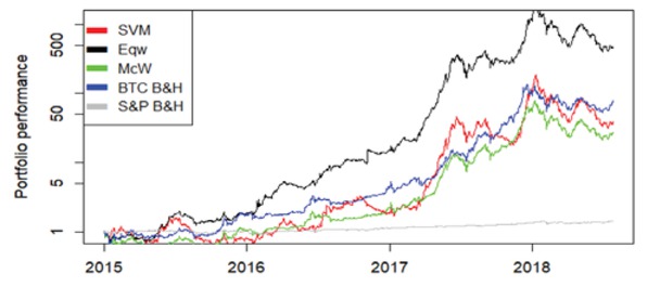
Fig. 4.1
The equity line of the SVM strategy in comparison with the benchmark strategies
Note: the graph shows equity lines of the SVM strategy and four benchmark strategies over the period from 01/01/2015 to 01/08/2018. EqW with equity line drawn in black outperforms all the benchmark strategies and also SVM strategy.
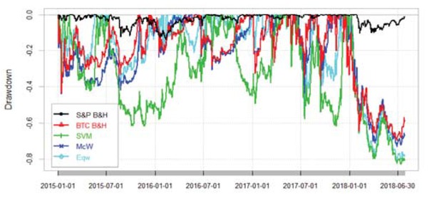
Fig 4.2
Drawdowns of the SVM strategy in comparison with the benchmark strategies
Note: the graph shows the drawdown lines for SVM strategy and four benchmark strategies over the period from 01/01/2015 to 01/08/2018. SVM strategy drawn in green reaches the ‘deepest’ drawdown line if compared to the other benchmark strategies.
Tab. 4.2
Descriptive statistics for SVM strategy (sensitivity analysis). Descriptive statistics for the benchmark strategies have been placed above for convenient comparison.
| Benchmark Strategies | ||||||||||
|---|---|---|---|---|---|---|---|---|---|---|
| Name | %ARC | %ASD | %MDD | IR1 | IR2 | %MT | ||||
| S&P B&H | 13.6 | 15.5 | 14.2 | 0.9 | 0.8 | |||||
| BTC B&H | 147.4 | 76.8 | 69.7 | 1.9 | 4.1 | 6.3 | ||||
| EqW | 425.8 | 96.2 | 81.7 | 4.4 | 23.1 | 10.8 | ||||
| McW | 141.9 | 74.9 | 73.1 | 1.9 | 3.7 | 6.3 | ||||
| SVM | 173.6 | 103.1 | 83.1 | 1.7 | 3.5 | 143.7 | ||||
| Parameters | SVM Strategy | |||||||||
| N | Position | %TS | RE | %TC | %ARC | %ASD | %MDD | IR1 | IR2 | %MT |
| 25 | long only | 50 | 3d | 1 | 19.4 | 108.7 | 90.6 | 0.2 | 0.0 | 115.3 |
| 25 | long only | 50 | 1w | 1 | 173.6 | 103.1 | 83.1 | 1.7 | 3.5 | 143.7 |
| 25 | long only | 50 | 1m | 1 | 224.2 | 101.5 | 86.0 | 2.2 | 5.8 | 148.8 |
| 5 | long only | 50 | 1w | 1 | -21.8 | 142.2 | 95.1 | -0.2 | 0.0 | 189.3 |
| 10 | long only | 50 | 1w | 1 | 89.3 | 131.7 | 85.0 | 0.7 | 0.7 | 176.8 |
| 15 | long only | 50 | 1w | 1 | 207.2 | 115.7 | 82.0 | 1.8 | 4.5 | 166.2 |
| 20 | long only | 50 | 1w | 1 | 215.9 | 110.0 | 82.3 | 2.0 | 5.1 | 154.3 |
| 25 | long only | 50 | 1w | 1 | 173.6 | 103.1 | 83.1 | 1.7 | 3.5 | 143.7 |
| VAR | long only | 50 | 1w | 1 | 326.4 | 92.6 | 57.6 | 3.5 | 20.0 | 105.6 |
| 25 | long only | 100 | 1w | 1 | 177.9 | 103.3 | 85.1 | 1.7 | 3.6 | 144.3 |
| 25 | long only | 50 | 1w | 1 | 173.6 | 103.1 | 83.1 | 1.7 | 3.5 | 143.7 |
| 25 | long only | 25 | 1w | 1 | 210.6 | 103.6 | 85.5 | 2.0 | 5.0 | 160.5 |
| 25 | long only | 50 | 1w | 0,5 | 368.8 | 110.2 | 76.5 | 3.3 | 16.1 | 155.4 |
| 25 | long only | 50 | 1w | 1 | 173.6 | 103.1 | 83.1 | 1.7 | 3,5 | 143.7 |
| 25 | long only | 50 | 1w | 2 | 29.6 | 110.9 | 88,1 | 0.3 | 0,1 | 154.9 |
| Best performance of SVM strategy with a selected set of parameters | ||||||||||
| N | Position | %TS | RE | %TC | %ARC | %ASD | %MDD | IR1 | IR2 | %MT |
| VAR | long only | 50 | 1m | 1 | 392.43 | 88.97 | 53.45 | 4.41 | 32.38 | 105.9 |
[i] Legend: McW – market cap weighted strategy, EqW – equally weighted strategy, N– number of currencies to be invested/used to construct portfolio, %TS – training data size, RE – the width of the reallocation period between the portfolio reallocation days, %TC – the total transaction costs taken as the percentage of the total transaction value of the portfolio, %ARC − annualized rate of return, %ASD − annualized standard deviation in percent, %MDD − maximum drawdown of capital in percent, IR1, IR2 − information ratios, %MT – the mean portfolio turnover ratio in percent.
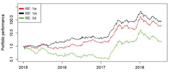
Fig. 4.3
Equity lines of the SVM strategy with changing reallocation period RE: 1 week (base case), 1 month and 3 days
Note: the graph shows the equity lines of the SVM strategy with changing reallocation period RE over the period from 01/01/2015 to 01/08/2018. The length of the reallocation period significantly impacts the portfolio performance.
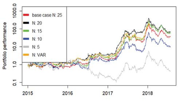
Fig. 4.4
Equity lines of the SVM strategy with changing number of assets N in the portfolio: 25, 20, 15, 10, 5 and VAR
Note: the graph shows the equity lines of the SVM strategy with changing number of assets N in the portfolio over the period from 01/01/2015 to 01/08/2018. The worst performance is noticed when only 5 coins are kept in the portfolio during a reallocation period. The lower the number of coins in the portfolio, the higher is the portfolio turnover.
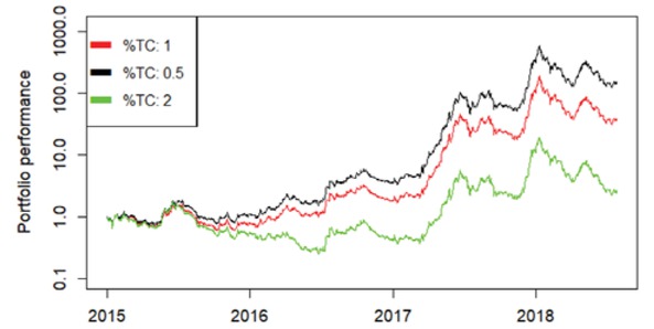
Fig. 4.5
Equity lines of the SVM strategy with various transaction costs (%TC equalled 2%, 1% and 0.5%)
Note: the graph shows the equity lines of the SVM strategy with changing transaction costs %TC in the portfolio over the period from 01/01/2015 to 01/08/2018. Performance of the portfolios heavily depends on the magnitude of transaction costs, which can be obviously seen from the behaviour of the equity lines.
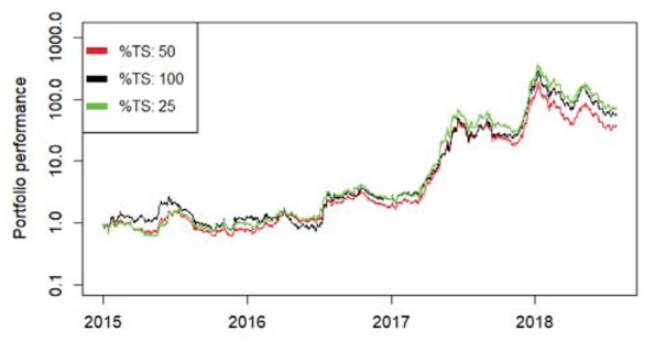
Fig. 4.6
Equity lines of the SVM strategy with changing length of the training set TS: 25%, 50%, and 100%
Note: the graph shows the equity lines of the SVM strategy with changing length of training set %TS in the portfolio over the period from 01/01/2015 to 01/08/2018. As lines are evolving very close to each other, one may conclude that the change of the parameter %TS does not exercise a significant impact on the portfolio statistics.