
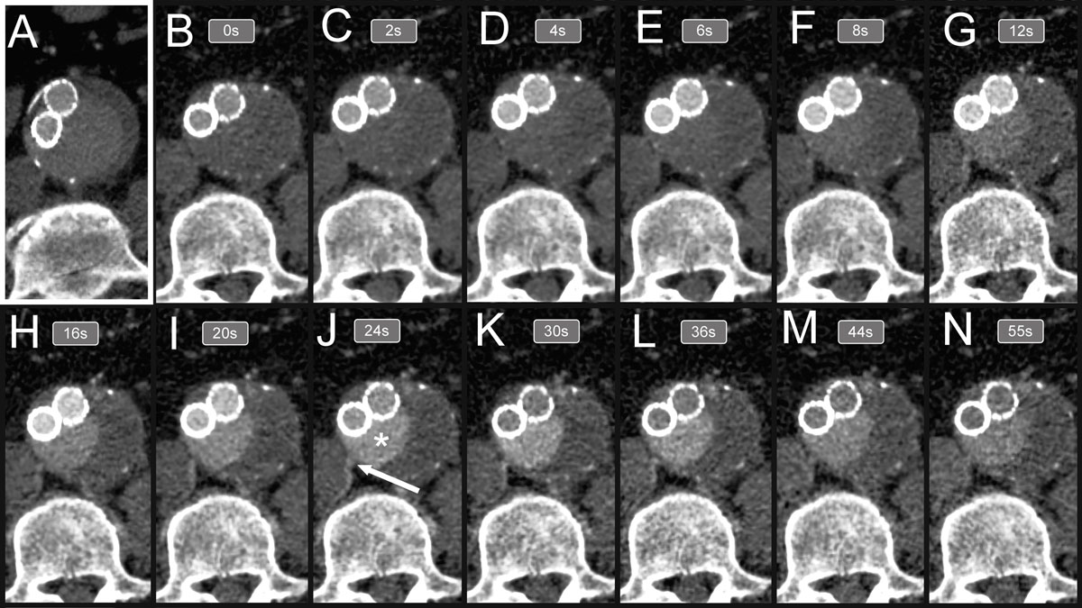
Figure 1
Delayed phase computed tomography (CTA) and dynamic CTA (d-CTA) images across multiple timepoints. During d-CTA, approximately 10 to 15 images are acquired in different timepoints after the contrast bolus to assess the exact type of endoleak. In this particular case, the most informative image is acquired around 24 seconds after contrast injections (panel J). The aneurysm sac (white * sign) is filled by the right lumbar artery (white arrow). In comparison, the image acquired with standard CTA in the delayed phase falls behind the acquired d-CTA images in terms of identifying the source of endoleak.
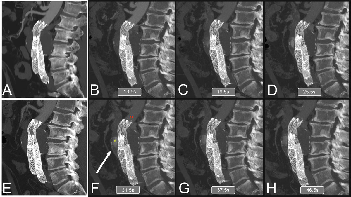
Figure 2
Comparison of arterial and delayed phases of triphasic computed tomography (CTA) with dynamic CTA findings. Compared to triphasic CTA, dynamic CTA is superior in identifying endoleak following endovascular aneurysm repair (EVAR). In this particular case, neither the arterial (A) nor the delayed (2 E) CTA phases were able to support endoleak as the underlying cause of progressive aneurysm sac growth following EVAR. In contrast, dynamic endoleak (panels B-D, F-H) was capable of showing the endoleak and the supplying inferior mesenteric artery (panel F, white arrow).
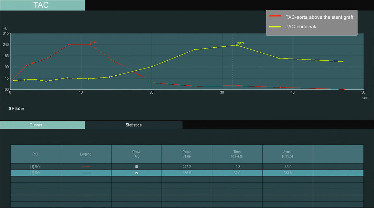
Figure 3
Time attenuation curve (TAC) of the aorta and the site of endoleak pertaining to Figure 2 dynamic CTA (d-CTA). The TAC of the d-CTA shows a significant delay (20 seconds) in the peak of the Hounsfield unit between the region of interest (ROI) placed in the aorta (red ° sign, ROI-1) and ROI placed at the site of the endoleak (yellow # sign, ROI-2), suggesting the sac filling from the inferior mesenteric artery toward the aneurysm sac rather than direct filling from the aorta.
Table 1
Dynamic computed tomography angiography imaging protocol for aortic endoleak detection. CT: computed tomography; CTA: computed tomography angiography; d-CTA: dynamic CTA
| DYNAMIC CTA IMAGING PROTOCOL FOR AORTIC ENDOLEAK | ||
|---|---|---|
| STEPS | DETAILED STEPS | |
| 1 | Patient positioning | Supine |
| 2 | Peripheral vein access | Right/left upper extremity |
| 3 | Topogram and noncontrast CT imaging acquisition | Sn-100 T in filter to reduce radiation exposure |
| 4 | Timing bolus to check contrast arrival time | 10-20 mL contrast injection followed by 50 mL saline at 3.5-4 mL/min flow rate, region of interest in aorta |
| 5 | Distribution and scan number planning | Choose DynMulti4D menu from the pop-up menu, plan distribution and scan number based on timing bolus and findings on previous studies |
| 6 | Optimize imaging parameters | To reduce exposure, optimize kV, scan range, etc. |
| 7 | Contrast injection for d-CTA acquisition | 70-80 mL contrast injection followed by 100 mL saline at 3.5-4 mL/min flow rate |
| 8 | Start d-CTA acquisition | Use delay time determined by the timing bolus |
| 9 | Parameters for d-CTA scan | 10-12 scans, tube voltage: 70-100 kV, tube current: 150 mAs, rotation time: 0.25 s, scan duration: 39 s, slice thickness: 0.7-1 mm, field of view (z-axis) : 23-33 cm |
Table 2
Dynamic magnetic resonance imaging protocol. MRI: magnetic resonance imaging; DICOM: Digital Imaging and Communications in Medicine; HASTE: half-fourier acquisition single-shot turbo spin-echo; PACS: picture archiving and communication system; SSFP: steady-state free precession; TWIST: time-resolved angiography with stochastic trajectories; VIBE: volumetric interpolated breath-hold examination
| DYNAMIC MRA PROTOCOL | ||
|---|---|---|
| STEPS | DETAILED STEPS | |
| 1 | Patient positioning | Supine |
| 2 | Peripheral vein access | Right/left upper extremity |
| 3 | Acquiring mask or later subtraction | Chest-abdomen noncontrast full-resolution image |
| 4 | Contrast administration | Gadolinium: 30-40 mL contrast material + 50 mL saline injection to wash out the contrast agent from the periphery Ferumoxytol (feraheme): 3 mL with 27 mL saline followed by 50 mL saline flush |
| 5 | Contrast passage visualization | Done by acquiring scan |
| 6 | Regular sequences are acquired for dynamic MRI scan | SSFP cine to evaluate dynamic vs static obstruction in TBAD HASTE, bright blood SSFP, 3D contrast-enhanced MRA to evaluate aortic morphology, TWIST for time resolved MRA, T1 VIBE for steady state imaging, 4D flow for qualitative and quantitative flow evaluation |
| 7 | 4D flow MRI | VENC 150-200 cm/s, acquisition time 7-12 min, free breathing |
| 8 | Send acquired data to database | Acquired data is sent to the institutional cloud-based imaging database (PACS) |
| 9 | Image analysis | Using DICOM viewer connected to the institutional PACS |
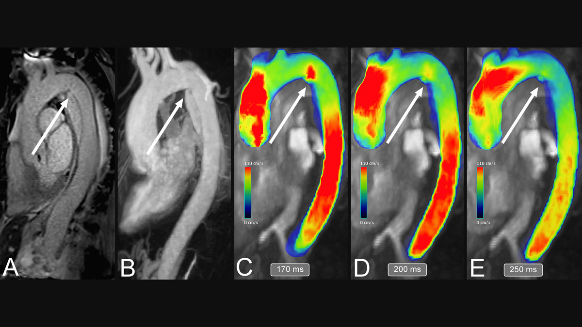
Figure 4
Qualitative analysis of type-B aortic dissection using magnetic resonance imaging (MRI). The contrast-enhanced MRA sequence (A) gives information on the site of the primary entry tear (white arrows), while the TWIST sequence shows the intimal flap and the directionality of false lumen filling (B). 4D flow MRI sequence (C-E) may complete the assessment of aortic dissection with color-coded velocity mapping, which is potentially able to uncover the tear where the false lumen is filling through (white arrows, C-E).
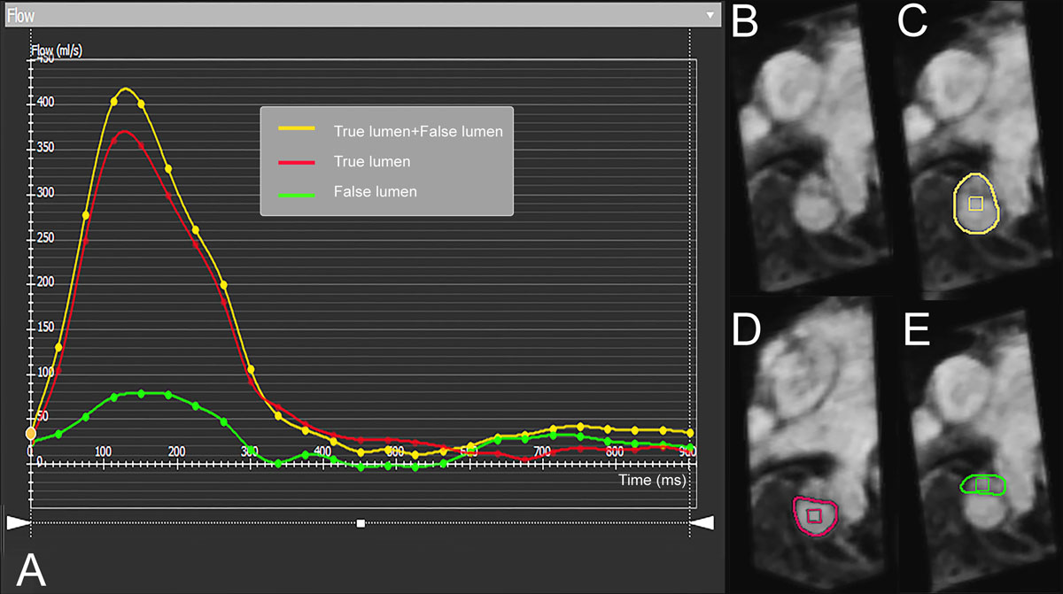
Figure 5
Quantitative flow evaluation of true lumen and false lumen using 4-dimensional (4D) flow magnetic resonance imaging (MRI). 4D flow MRI provides quantification of flow parameters depicted by the marked areas on panels B-E. The flow volume is displayed in a graph (A) where the y-axis represents the flow volume (mL/s) through the marked area and the x-axis represents time in milliseconds. In aortic dissection, the true lumen (A: red line, D: red outline) and the false lumen (A: green line, E: green outline) can be interrogated, and the entire flow volume (A: yellow line, C: yellow outline) can be determined.