
Introduction
Contemporary research on river systems increasingly incorporates the analysis of channel position and morphology, both of which undergo continuous transformations driven by variable hydrodynamic conditions. Channel morphology plays a fundamental role in the hydrological and morphodynamic processes, directly influencing water flow, sedimentation and sediment transport. The analysis of water-covered areas and floodplains is crucial not only for hydrological and geomorphological studies but also in the context of flood risk management and emergency planning (Sanyal, Lu 2004, Schumann et al. 2011, Du et al. 2012, Kuenzer et al. 2013, Hojan, Rurek 2021, Wierzbicki et al. 2021, Ghosh et al. 2023). Alterations in river channel structure can result in the redirection of flow paths, thereby increasing flood risk or affecting the effectiveness of protective measures (Burshtynska et al. 2016, 2017, Kumar Pal et al. 2017, Rashid, Habib 2022, Hossain et al. 2024). Therefore, continuous monitoring of these processes is essential for developing effective environmental management strategies and spatial planning in river valleys.
Although numerous field-based and remote sensing analyses are currently being conducted, there remains a pressing need to improve monitoring tools and methodologies to better predict changes in river systems and more effectively mitigate the adverse impacts of extreme hydrological events. A breakthrough in water-related research has been the increased accessibility of satellite data, which enables large-scale analyses with significantly reduced labour intensity through the application of remote sensing techniques.
Water, compared with other landforms, absorbs a significant portion of electromagnetic radiation. Pure water has a spectral reflectance maximum, albeit very low, in the green range. Practically all of the energy is absorbed in the near-infrared (NIR) and far infrared ranges (Bartolucci et al. 1977). The albedo of pure water is approximately in the range 0.03–0.1 and varies depending on the type and amount of so-called optically significant substances (OSS) (Dworak et al. 2011). These include total suspended solids (TSS), coloured dissolved organic matter (CDOM) and chlorophyll. As the amount of OSS increases, the albedo increases too, and the water appears brighter in aerial and satellite images (Osińska-Skotak 2010, Dworak et al. 2011). Based on these properties of water and the suspensions contained in it, many spectral indices have been developed to detect surface waters and their quality. To detect water bodies, McFeeters (1996) introduced the Normalized Difference Water Index (NDWI), utilising green and NIR bands. Although effective in highlighting water features, NDWI is sensitive to built-up areas, often overestimating water extent. Xu (2005, 2006) improved this by proposing the modified Normalized Difference Water Index (MNDWI), replacing the NIR band with shortwave infrared (SWIR). Feyisa et al. (2014) introduced the Automated Water Extraction Index (AWEI), which has two variants for better water differentiation in the presence of very bright objects (snow) or deep shadows cast by mountains, buildings or trees in the analysed scene. Building on these approaches, the sentinel water mask (SWM) index was developed for Sentinel-2 top-of-atmosphere (TOA) data (Robak et al. 2016), using green, blue, NIR and SWIR, which was successfully used by Kryniecka and Magnuszewski (2020, 2021) to study alternate sandbars movement at the Vistula River, Poland. The literature provides numerous additional examples of water indices, which are particularly valuable for studying the dynamic processes of river channels that shape the geomorphology and ecosystems, especially in the context of extreme hydrological events such as floods. These indices have been widely applied in studies primarily focused on large river systems or water reservoirs (Ji et al. 2009, Dworak et al. 2011, Li et al. 2013, Du et al. 2014, Sarp, Ozcelik 2017, Yang et al. 2017, Acharya et al. 2018, Pereira et al. 2018, Wang, Jun Xu 2018, Ali et al. 2019, Hejmanowska et al. 2020, Kryniecka, Magnuszewski 2020, Khan 2022, Laonamsai et al. 2023, Borkowski et al. 2024, Le et al. 2024). Pluto-Kossakowska et al. (2018) demonstrated the high usefulness of Sentinel-2 images for detecting small water bodies. A separate group of indices are those intended for testing water quality (see e.g. Osińska-Skotak 2010, Dworak et al. 2011, Simiyu, Mwatelah 2025). Although they are not the subject of our research, it should be noted that the presence of OSS in the water, as well as water depth, by influencing the representation of water in images, significantly impacts the accuracy of detecting morphological details in rivers. The representation of water bodies in remote sensing data also depends on water depth, the type of material covering the bottom, and the direction of illumination and observation (Albertz 2007). The latter two factors are particularly important in airborne remote sensing. In the case of satellite remote sensing, the state of the atmosphere is important because it scatters or absorbs (to varying degrees) electromagnetic radiation, including those ranges that are important for water detection. Pure water reflects a small amount of incident electromagnetic radiation, with a peak in the blue wavelength range. However, it absorbs all infrared radiation. The scattering of radiation in the atmosphere causes an increase in the radiation values recorded by the sensor, especially in the shorter wavelength ranges. This deepens the difference between the recorded (B + G) and NIR reflectance values. All other objects on the Earth’s surface exhibit significant reflection (compared with water) in the NIR and far infrared ranges, well above atmospheric noise. Therefore, water remains the darkest object (especially in the infrared range) and is easily distinguished both visually and by indices. Correcting the radiance to the ground level (bottom of atmosphere) is considered an important step in the water detection process (Dworak et al. 2011, Ning, Lee 2012, Acharya et al. 2018, Trinh et al. 2024, Simiyu, Mwatelah 2025). There are many methods of atmospheric correction, and satellite data providers also offer appropriately processed data. However, as Osińska-Skotak (2010) writes, they use so-called models of average atmospheric climates, which may not represent the conditions prevailing at the time the images were recorded. There are also approaches that use uncorrected images (Yang et al. 2017) or even consider such images to be better. Robak et al. (2016) and Pan et al. (2020) found that the L1C level images are better than corrected ones. This was probably due to the fact that the correction method used was not entirely appropriate. Kryniecka and Magnuszewski successfully used Sentinel-2 images from both L2A (2020) and L1C (2021). The authors of some works do not provide any information about the status of the processed images in this context (Kupidura 2013, Sarp, Ozcelik 2017). This approach has its justification, since spectral indices, as arithmetic operations on spectral channels, represent their mutual relationships rather than absolute values. Therefore, they allow many problems to be bypassed, such as sensor calibration, changing radiation conditions, atmospheric conditions and so on (Lei et al. 2009). Compared with spectral characteristics, spatial resolution is much more important in water identification, particularly the presence of image pixels containing mixed spectral responses from the water and its surroundings. In our conditions, these include bright sandbars and vegetation (e.g. grasses, shrubs and trees).
The image processing process for water detection basically has three main stages (Pan et al. 2020): 1. Calculation of indices, 2. Binary division of the study area into water and non-water bodies using various algorithms and 3. Accuracy assessment based on ground-truth data. Spectral indices are most often analysed separately when the goal is to detect water bodies. However, they can be combined into a single equation when the goal is to determine a single, resulting water quality index that takes into account the synergy of various water characteristics (Simiyu, Mwatelah 2025). This latter approach (Acharya et al. 2018), however, appears to be unpopular in water extent detection. The purpose of water detection is to highlight two areas in the images: water and non-water. To achieve this result, methods of varying degrees of technological advancement are used: visual interpretation, thresholding of single channels or spectral indices, pixel-based and object-based classification, including texture analysis, mathematical morphology and spectral mixture analysis (Lei et al. 2009, Ning, Lee 2012, Kupidura 2013, Robak et al. 2016, Kaplan, Avdan 2017, Yang, Du 2017). The final step, assessing the accuracy, requires appropriate reference data. However, even in countries with appropriate geospatial databases, this may be impossible due to the dynamics of river course changes, which are not matched by the frequency of relevant field measurements. Therefore, analyses often involve searching for changes between two or more points in time or using point-based ground-truth samples.
The water detection methods developed for specific test areas do not always perform equally well under different geographic conditions, emphasising the need for their validation across diverse environments. Such an approach enables a more comprehensive assessment of their effectiveness and enhances the potential for optimal selection of research tools – an essential step for the continued advancement of remote sensing methodologies.
The aim of this study is to evaluate the effectiveness of three selected water indices (SWM, NDWI, MNDWI) for the detection of surface water and for the analysis of changes in water bodies based on Sentinel-2 Level 1C satellite imagery in a temperate climate. The indices were compared in several test areas that included both the main channel of a large river (the Vistula) and significantly smaller tributaries and minor water bodies. Studies on the condition of the Vistula River bed using remote sensing methods were conducted, among others, by Trafas (1975, 1977), Babiński (1984), Wilczyński et al. (1994), Dobrowolski et al. (2004), Kryniecka and Magnuszewski (2020, 2021) and focused mainly on the main body of the river. Changes in the beds of other rivers were previously successfully studied using aerial photographs by, among others, Baraniecki and Ruszczycka-Mizera (1977), Florek (1983), Śmielak (2008) and Tobiasz (2012). Although these studies were conducted from different altitudes (namely, aerial and satellite) and under various natural conditions, the high usefulness of remote sensing images for recording and interpreting the course of morphological processes in rivers was confirmed.
To assess the suitability of the Sentinel 2 L1C images and indices used in our study for temporal variability analysis, the study was conducted over a time span from 2019 to 2022 for the same regions.
Study area
To test the performance of spectral indices in detecting water in both large rivers and significantly smaller streams, two study areas located in the temperate climate zone of Poland were selected for analysis. These areas include the main channel of the Vistula River and several of its tributaries. The Vistula River is the longest in Poland (1047.5 km – Łajczak et al. 2021), originating in the Silesian Beskids on the slopes of Barania Góra (1220 m a.s.l.), and flowing into the Baltic Sea (Dajek et al. 2011). The key characteristics of the river are presented in Table 1.
Table 1.
Selected characteristics of the Vistula River (Łajczak et al. 2021).
| Characteristic of the Vistula River | Value |
|---|---|
| Drainage basin area | 194,424 km2 |
| Valley length | 525 km |
| Average discharge at the mouth | 1,080 m3/s |
| Amount of transported suspended and bedload material | 833,000 t/year |
| River sinuosity | 115% |
The study was conducted within two selected research areas traversed by the middle Vistula River, which represents approximately 270 km of the total length of the river. This begins at the confluence with the San River and extends northward to the confluence with the Narew River (Fig. 1A). The average discharge below the Narew confluence reaches 950 m3 · s-1 (Łajczak et al. 2021). Initially, the Vistula River flows through a lowland area; from Annopol, it traverses approximately 80 km of upland terrain before entering the Mazovian Lowland.
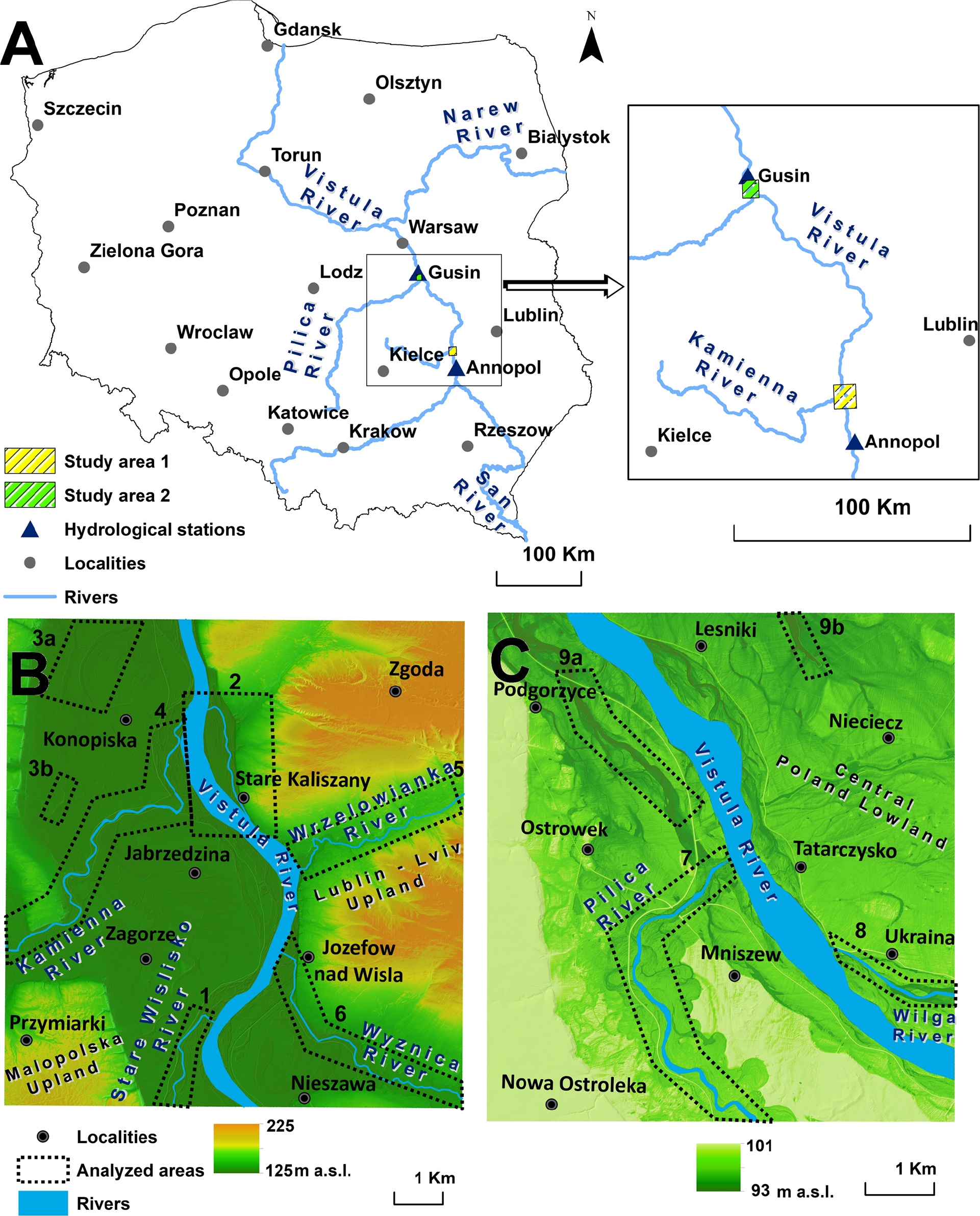
Fig. 1.
Study area. A – Location of research areas in Poland; positions of hydrological stations are marked with triangles; B – Physical-geographical map of Research Area 1 with designated test areas; C – Physical-geographical map of Research Area 2 with designated test areas; based on data from GUGiK – www.geoportal.gov.pl/.
Research Area 1 (Fig. 1B) is situated within the Małopolska Upland and the Lublin–Lviv Upland. The valley in this region can be characterised as symmetrical and narrow, with a relatively gentle river gradient. The analysis covered an area defined by a polygon measuring 9.5 by 10 km (Fig. 2 – RA 1). The primary tributary of the Vistula River in this section is the Kamienna River (confluence at 324 km of the Vistula River), with smaller tributaries including the Wyznica and Wrzelowianka Rivers. Within the floodplain of the Vistula River, two former channels of the river are present and are currently partially water-filled: Stare Wislisko and an abandoned channel near the village of Stare Kaliszany.
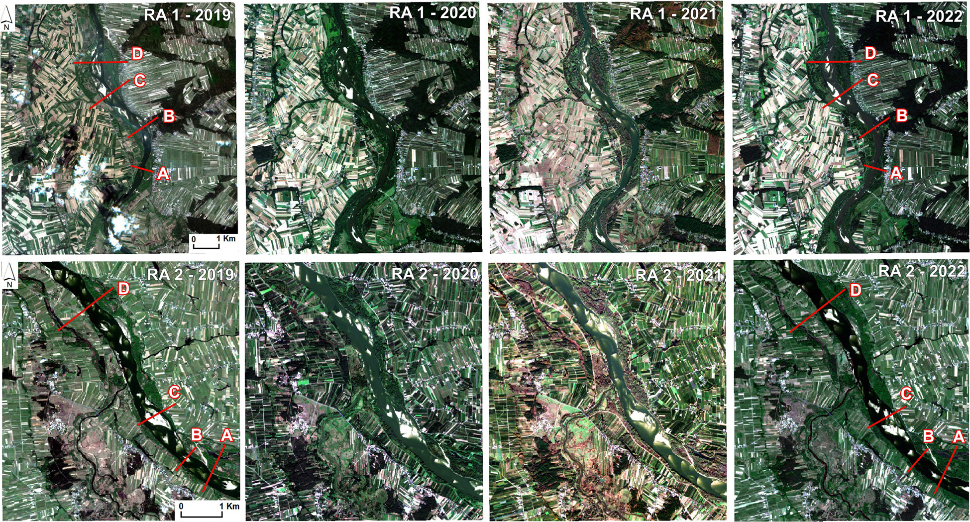
Fig. 2.
RGB composites for Research Areas 1 and 2; A–D – profile lines drawn through the analysed spectral indices, shown in Figures 8 and 9.
Research Area 2 (Fig. 1C) is located approximately 90 km north of Area 1 in a straight line. The area analysed encompasses a polygon measuring 6.9 by 7.4 km (Fig. 2 – RA 2). The main tributary within this section is the Pilica River (which joins the Vistula River at 457 km), along with the smaller Wilga River. Hydrological monitoring stations are located near both study areas in Annopol (298 km) and Gusin (461 km). The channel width of the Vistula River within the studied sections varies from approximately 200 to 800 m.
Extensive sandy mid-channel bars are present along significant segments of the river within both research areas (Fig. 2). Within Research Area 1, seven smaller test areas (1–6) were delineated for a more detailed analysis, while Research Area 2 includes four test areas (7–9). Their locations are presented in Figure 1B, C.
Materials and methods
Data collection
The satellite imagery used as the basis for this study was acquired under the Copernicus Programme, conducted as part of the ESA Sentinel mission, managed by the European Space Agency. The images were captured by the multi-spectral instrument (MSI) onboard Sentinel-2A satellite, which records data across 13 spectral bands, including visible (VIS) and (NIR and SWIR) wavelengths. The analyses were conducted for two research areas using imagery acquired between 2019 and 2022.
The selection of satellite scenes was based on strictly defined criteria. In studies of river valley morphodynamics, it is essential to analyse changes using data acquired under comparable conditions. This required identifying images in which the water levels in the Vistula River during the study period were as similar as possible. Therefore, the selection process began with an analysis of data from hydrological stations operated by IMGW-PIB, located closest to the study sections of the river – in Annopol (14 km south of Research Area 1) and in Gusin (3 km north of Research Area 2). Among the available data, the most frequently recurring water levels were identified, followed by the selection of those that were lower than the annual average. This approach provided better visibility of the sandbars and their morphological features than would have been possible under higher water conditions. Subsequently, scenes were selected with water levels as similar as possible. The selection process also considered the temporal resolution of Sentinel-2A and 2B satellite overpasses (10 days) and the atmospheric conditions at the time of acquisition. Ultimately, one scene per year (2019–2022) was selected for each study section, resulting in a total of eight Sentinel-2A images (Table 2). Level 1C data (TOA reflectance) were used, as this type of imagery, according to Robak et al. (2016), allows for more precise water detection than atmospherically corrected images.
Table 2.
List of Sentinel-2 satellite scenes used in the analysis with corresponding water levels and stage classification.
| Study area | Photo date | Satellite scene name | Water level | Stage zone |
|---|---|---|---|---|
| 1 | 25.04.2019 | S2A_MSIL1C_20190425T094031_N0207 | 215 cm | low |
| 1 | 22.08.2020 | S2B_MSIL1C_20200822T094039_N0500 | 220 cm | low |
| 1 | 31.10.2021 | S2A_MSIL1C_20211031T094141_N0500 | 219 cm | low |
| 1 | 27.08.2022 | S2A_MSIL1C_20220827T093601_N0400 | 211 cm | low |
| 2 | 25.04.2019 | S2A_MSIL1C_20190425T094031_N0207 | 50 cm | low |
| 2 | 14.09.2020 | S2B_MSIL1C_20200914T095029_N0500 | 57 cm | low |
| 2 | 29.10.2021 | S2B_MSIL1C_20211029T095029_N0301 | 60 cm | low |
| 2 | 19.05.2022 | S2A_MSIL1C_20220519T094041_N0400 | 61 cm | low |
Data processing
The mathematical formulas of the selected indices are based on the following bands: blue (2), green (3), NIR (8) and SWIR (11). The data processing began with resampling the spectral bands to ensure a consistent spatial resolution. Bands 2, 3 and 8 have Ground Sampling Distance GSD = 10 m, while band 11 has GSD = 20 m. Therefore, band 11 was resampled to 10 m to ensure consistency by simply dividing the pixels into smaller ones to avoid changes in pixel values. Subsequently, the scenes were clipped to match the research areas. GIS software ArcMap version 10.4.1 was used to conduct the analyses. The overall data analysis process is illustrated in Figure 3. The next stage of data processing involved the calculation of three selected water indices: NDWI, MNDWI and SWM (Table 3). This was done using the Raster Calculator tool. As a result, raster products were generated, with grid cells recalculated to reflect new values. Visualisations of the computed indices are shown in Figures 4 and 5. In the derived indices, the value ranges were as follows: NDWI: -0.7 to 0.6, MNDWI: -0.7 to 1 and SWM: 0.2–6. High grid cell values indicated the presence of water, while low values corresponded to other land cover types.
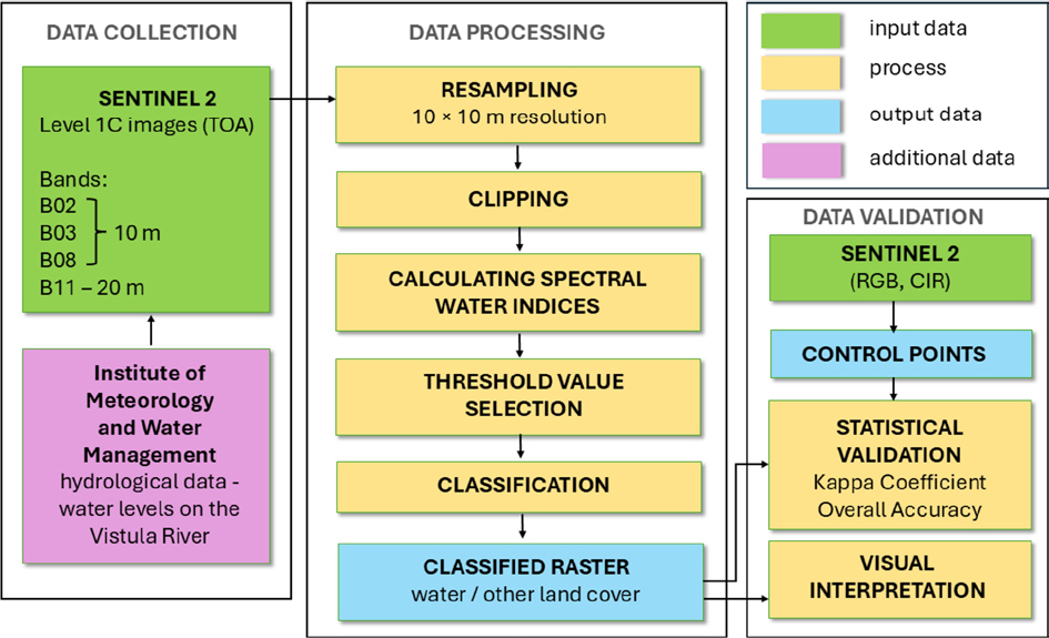
Fig. 3.
Diagram of the data analysis process.
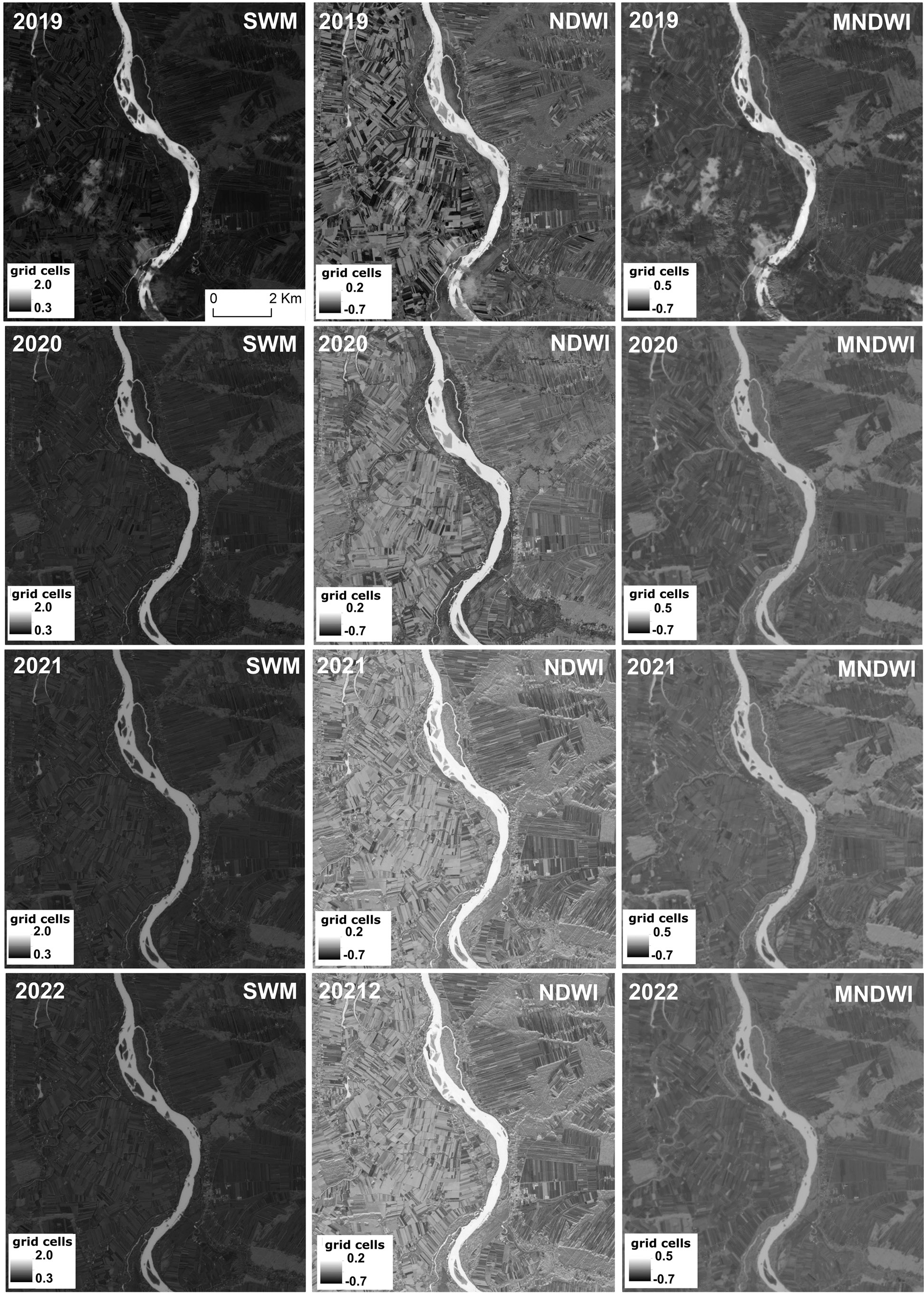
Fig. 4.
Water index maps for Research Area 1.
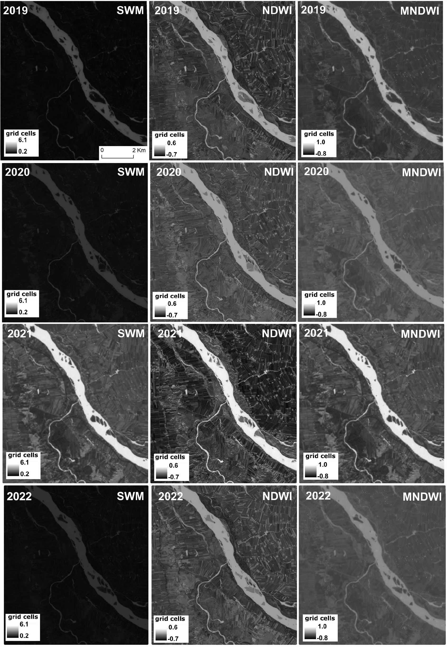
Fig. 5.
Water index maps for Research Area 2.
Table 3.
Basic characteristics of the applied spectral indices.
| Water Index | Equation | Reference |
|---|---|---|
| Normalized Difference Water Index (NDWI) | NDWI = (Green - NIR)/(Green + NIR) | McFeeters (1996) |
| Modified Normalized Difference Water Index (MNDWI) | MNDWI = (Green - SWIR)/(Green + SWIR) | Xu (2006) |
| the Sentinel Water Mask (SWM) | SWM = (Blue + Green)/(NIR + SWIR) | Robak et al. (2016) |
In the next stage of the study, manual thresholding of the calculated indices was performed. This process involved determining a grid cell value that served as the boundary between water and other types of land cover. Thresholding was conducted separately for each raster, since, despite normalisation of grid cell values through the calculation of spectral indices, the resulting value ranges were not identical. The imagery differed in minimum and maximum grid cell values due to varying satellite acquisition conditions, such as weather, solar angle and differences in land cover between research sections 1 and 2. The thresholding was performed using the Reclassify tool by dividing grid cells into two classes: ‘water’ and ‘other land cover’. This was done based on histogram analyses, which showed the frequency distribution of individual grid cell values in the images. The optimal threshold value, most accurately separating water from the surrounding environment, was identified at the inflection point on the histogram. The result of the analysis was a set of 24 classified raster files, which are presented in Figures 6 and 7.
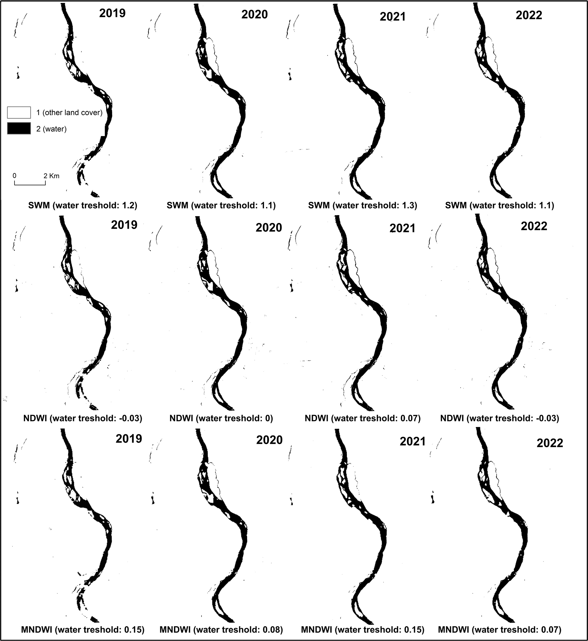
Fig. 6.
Thresholded spectral indices for Research Area 1.
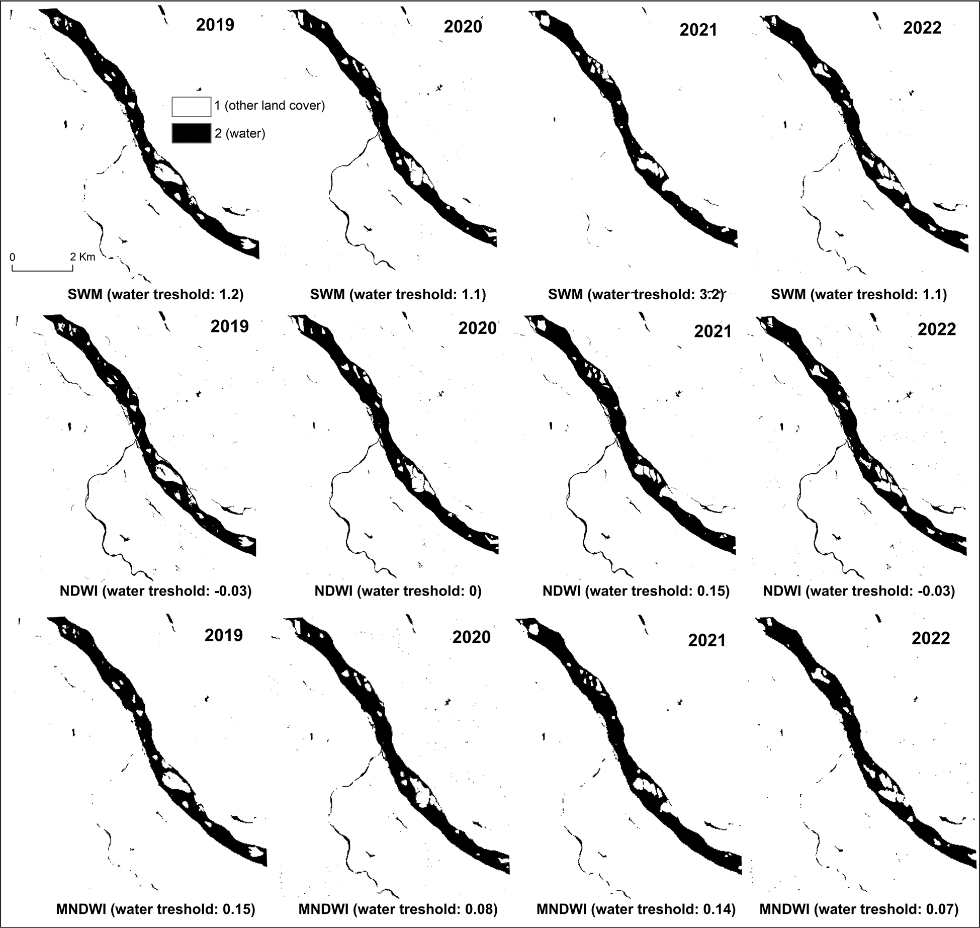
Fig. 7.
Thresholded spectral indices for Research Area 2.
To evaluate the annual variability of the NDWI values, Sentinel-2 scenes from 2019, 2020, 2021 and 2022 were analysed using the Copernicus Browser. Image selection was constrained by a maximum cloud-cover threshold of 20%, ensuring the use of scenes with sufficient surface visibility. Data were analysed for the full annual cycle, covering the period from the beginning to the end of each year. The analysis focused on selected polygons located within the Vistula River channel that represented water bodies throughout the entire study period. Only areas that remained continuously inundated were considered, in order to ensure temporal consistency and to eliminate the influence of seasonal changes in channel position or exposed bars. The plots showing the annual evolution of NDWI were developed based on mean grid cell values calculated from the polygons for each research area.
Data validation
To compare the accuracy of the applied indices, a validation procedure based on control points was conducted. For each of the two study areas, 500 validation points were added, and each was manually assigned the attribute ‘water’ or ‘other land cover’. The classification was based on RGB (bands 2, 3, 4) and CIR (bands 3, 4, 8) composite images, which were composed from the same Sentinel scenes that were used for the calculation of spectral indices. Of the total points, 300 were randomly distributed, while 200 were manually selected, with a focus on water bodies and urbanised areas, which are particularly difficult to distinguish from water. The manually defined classes were compared with the grid cell values derived from the raster layers of the calculated indices. Subsequently, a statistical analysis was carried out to evaluate classification accuracy by calculating overall accuracy, user accuracy, producer accuracy and the kappa coefficient.
Additionally, to enable more detailed analysis of smaller watercourses and water bodies, 11 smaller test areas were selected for visual assessment (Figs 1A, B, 11, 15), encompassing all visible water bodies within the research areas. The accuracy of the water representation was compared between the RGB and CIR images and the calculated NDWI, MNDWI and SWM indices for each analysed area within the 2019–2022 time frame. Cross-sections were established across the Vistula River, four in each of two locations: Research Area 1 (Fig. 8) and Research Area 2 (Fig. 9). The cross-sections run through three landcover classes: water, river bars and riparian vegetation. The variability of the index values in these characteristic landcover types was also examined. For this purpose, 240 points were designated, 80 for each landcover type, in whose vicinity index values were collected from 9 grid cells and then averaged. The ranges of the resulting values are presented in Figure 10. By comparing the image series presented in Figures 12–14 and 16–18, the effectiveness of each spectral index was assessed over four different years, as well as the comparative performance of three different indices on a single image from 1 year. The results of the evaluation for the detection of water using the selected indices are presented in Tables 5 and 6. A three-point rating scale was applied: 1/2/3, where 1 indicates the lowest accuracy, 2 indicates moderate accuracy, and 3 indicates the highest accuracy in detecting water features. Subsequently, the frequency of specific ratings assigned by the indices was analysed, and their effectiveness was estimated as the percentage of points obtained.
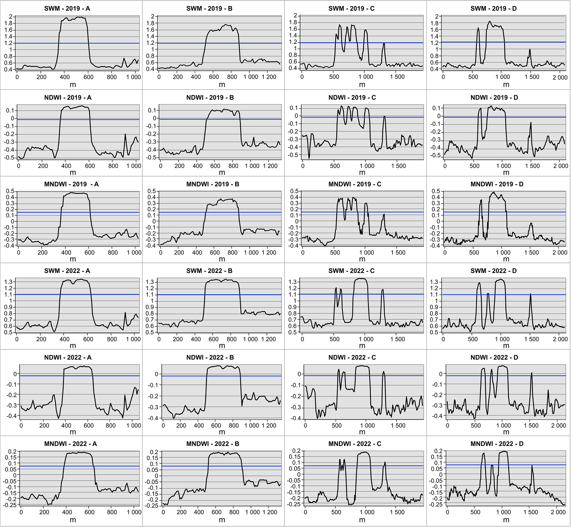
Fig. 8.
Cross-sections across the Vistula River in Research Area 1, running through three land-cover classes: water, river bars and riparian vegetation. The location of the profiles is shown in Fig. 2. The blue line indicates the adopted threshold value.
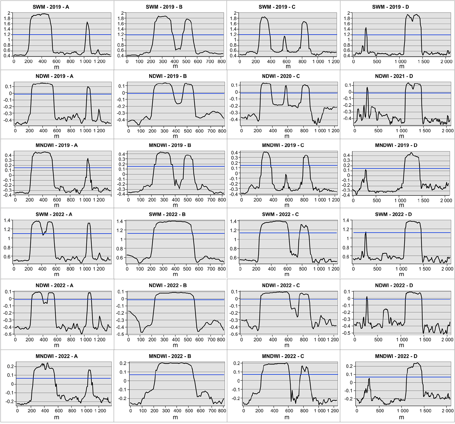
Fig. 9.
Cross-sections across the Vistula River in Research Area 2, running through three land-cover classes: water, river bars and riparian vegetation. The location of the profiles is shown in Fig. 2. The blue line indicates the adopted threshold value.
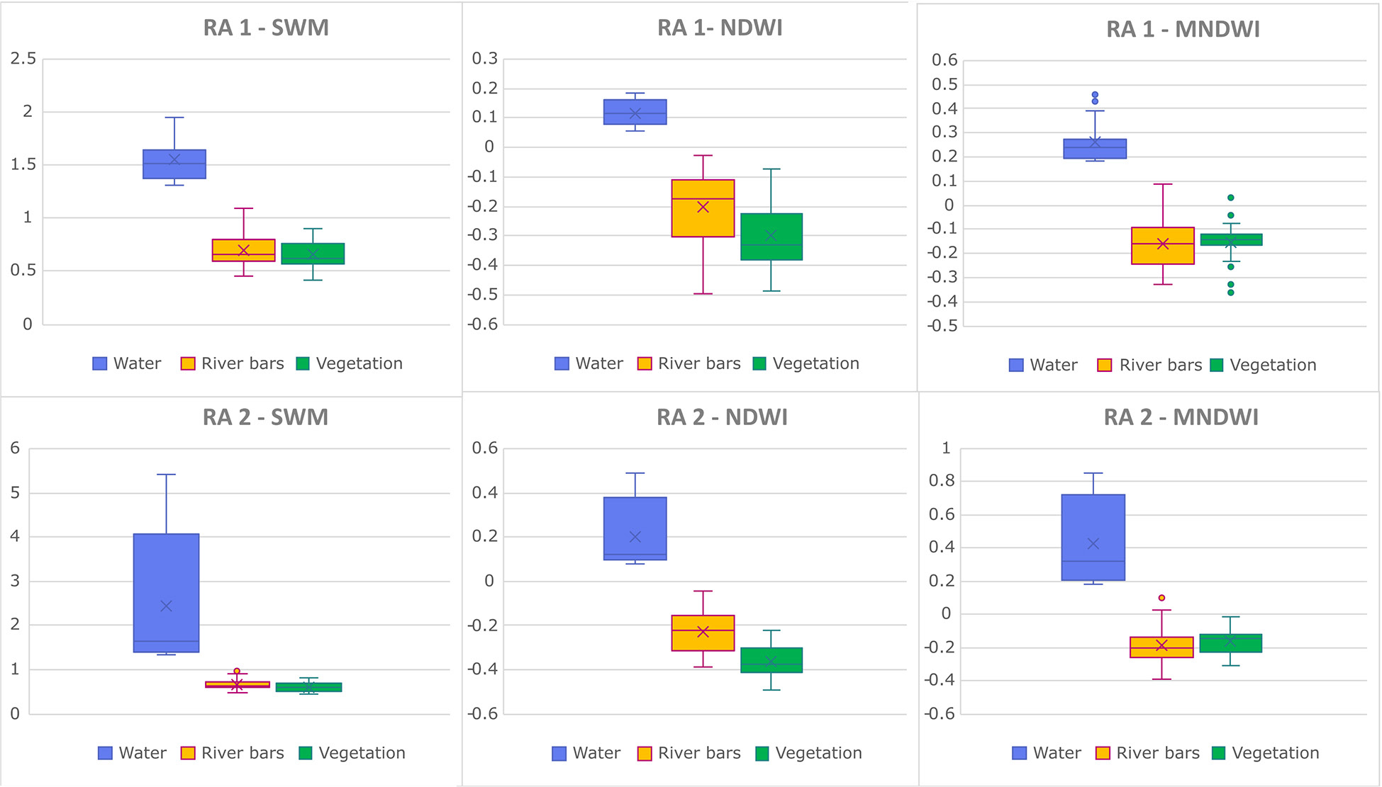
Fig. 10.
Diagram presenting the variability of indices values within three land-cover classes: water, river bars and riparian vegetation.
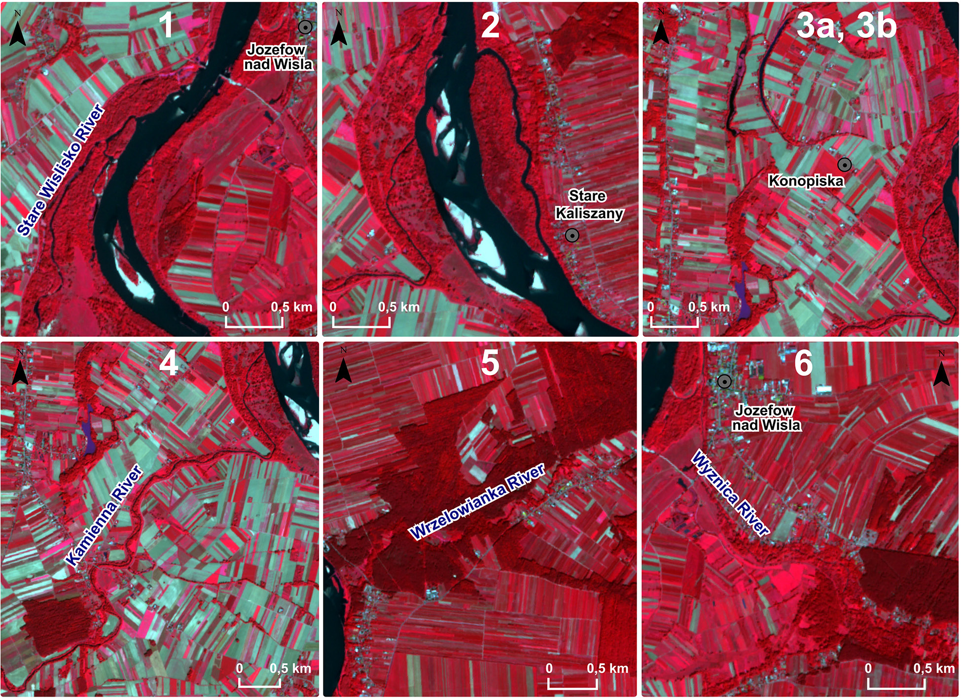
Fig. 11.
Selected test areas within Research Area 1 in the CIR composition in the year 2022.
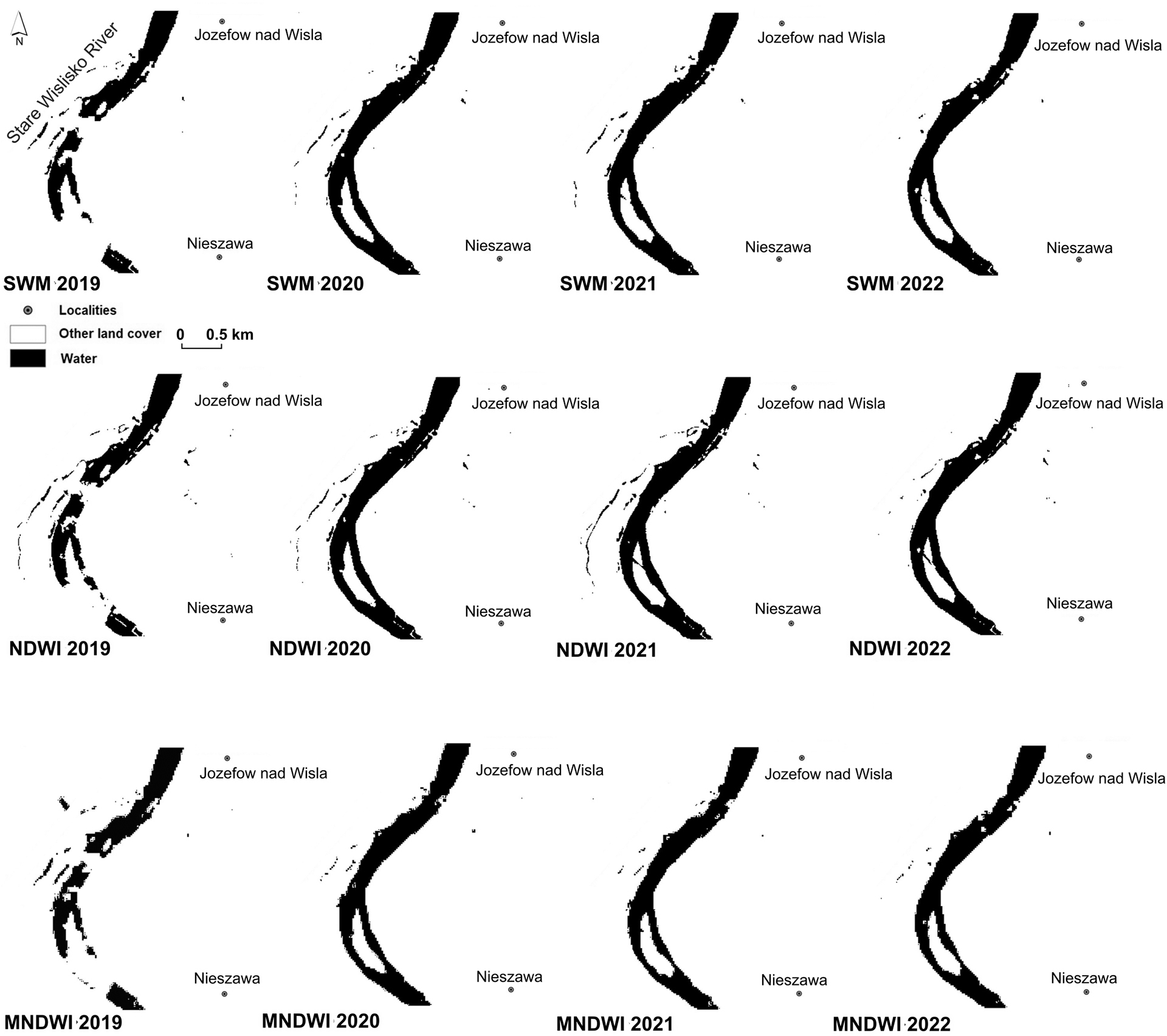
Fig. 12.
Thresholded water indices for test area 1 (Stare Wislisko) in the years 2019–2022.
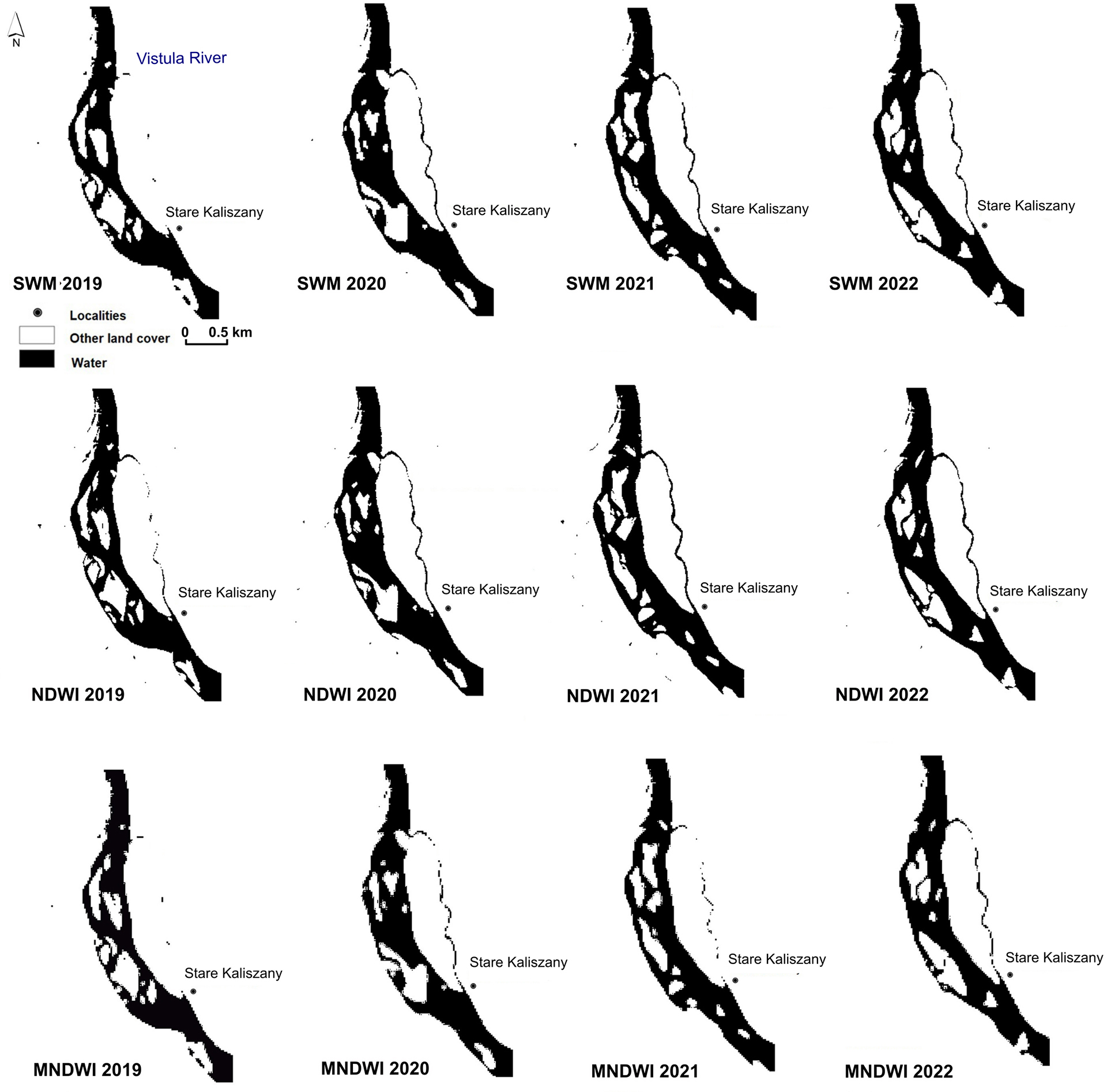
Fig. 13.
Thresholded water indices for test area 2 (branch of the Vistula River) in the years 2019–2022.
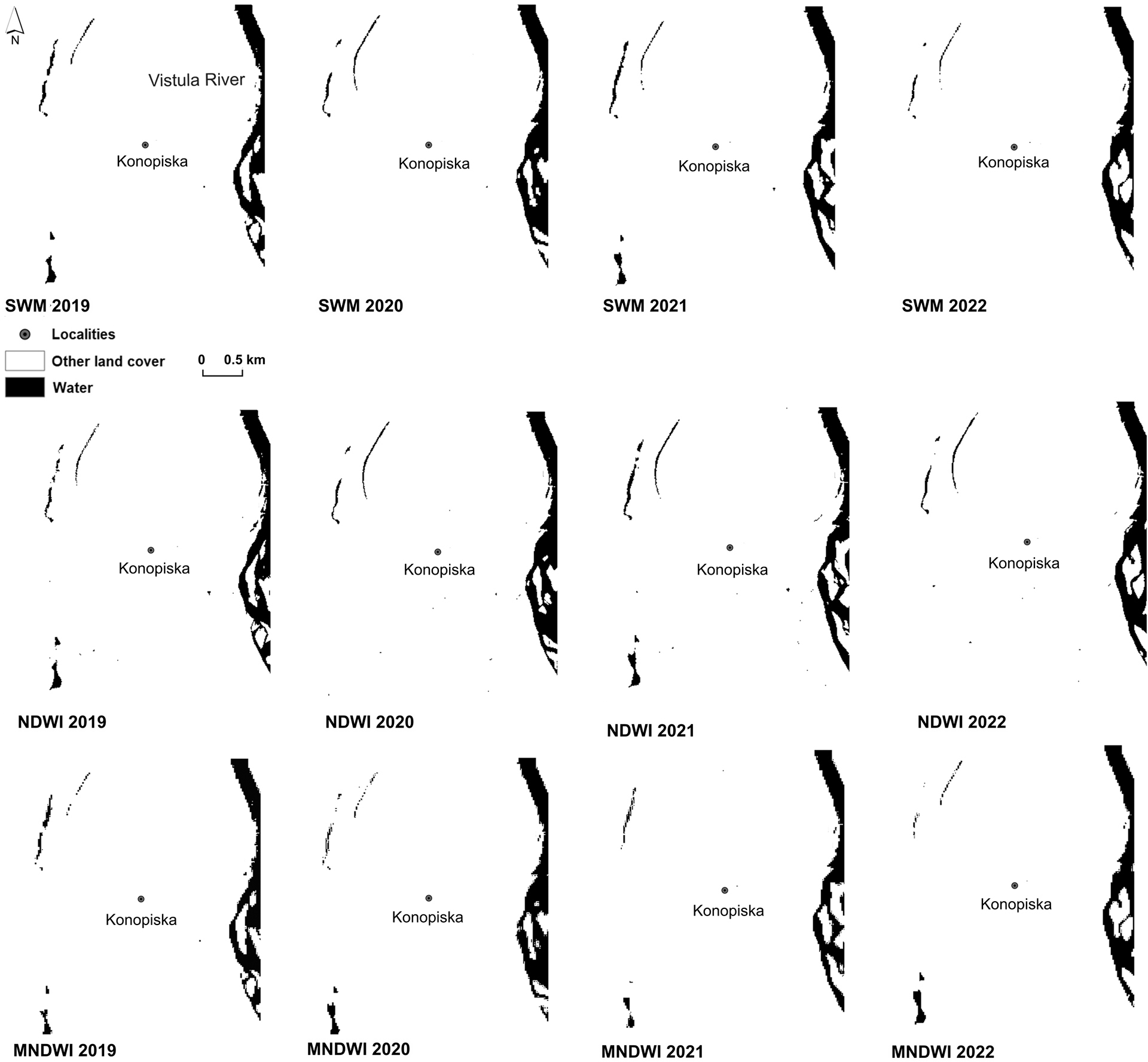
Fig. 14.
Thresholded water indices for test areas 3a and 3b (an example of water bodies in Research Area 1) in the years 2019–2022.
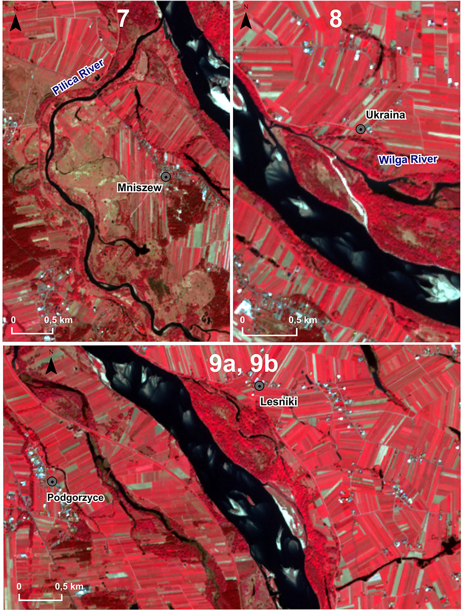
Fig. 15
Selected test areas within Research Area 2 in the CIR composition in the year 2022.
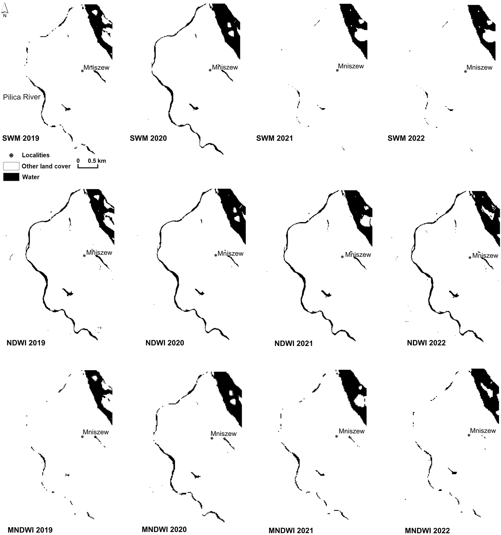
Fig. 16.
Thresholded water indices for test area 7 (Pilica River) in the years 2019–2022.
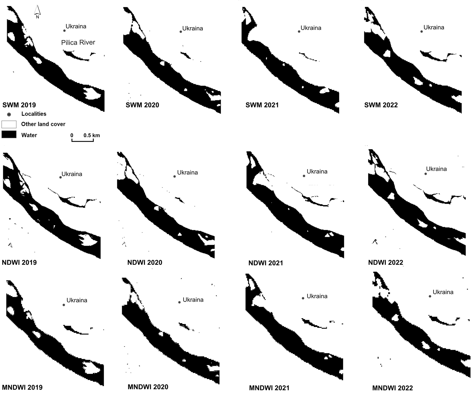
Fig. 17.
Thresholded water indices for test area 8 (Wilga River) in the years 2019–2022.
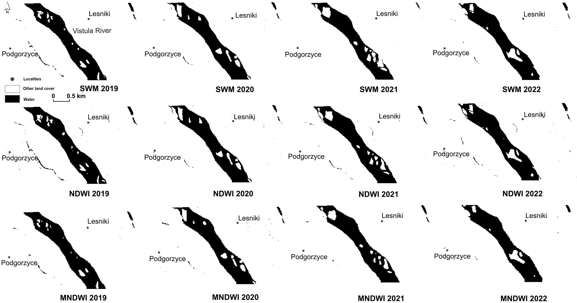
Fig. 18.
Thresholded water indices for test areas 9a and 9b (an example of water bodies in Research Area 2) in the years 2019–2022.
Results and discussion
Based on the calculated spectral indices (Figs 4 and 5) and the raster layers generated after thresholding these indices (Figs 6 and 7), an analysis was conducted to assess the accuracy of the results and determine whether any of the applied indices yielded better outcomes than the others. Preliminary observations indicated that SWM, NDWI and MNDWI accurately reflected the actual condition of surface water within the main river channel. In each figure, the Vistula River was clearly delineated. This means that the water mask corresponded well with the real location and layout of the riverbed. In the case of Research Area 1, the characteristic meanders are visible (Fig. 6), while Research Area 2 reveals a more braided river pattern (Fig. 7).
The successful detection of water is attributed to the fact that, in the calculated indices, the Vistula River exhibited high grid cell values, which made it stand out as a bright object compared with the surrounding land cover. In Figures 8 and 9, the water/non-water boundary transitions are clearly visible, that is, water with coastal vegetation and water with sandbars. The ranges of index variability (in box plots, Fig. 10) also show that water clearly differs in terms of index values from the other two land cover forms, sandbars and vegetation, with the NDWI index demonstrating the best differentiation. This pattern, combined with appropriately selected threshold values, resulted in a water mask that accurately represents the length, width and shape of the Vistula River.
Selected test areas were analysed at a larger scale to verify whether, beyond detecting the general course of the Vistula River, other rivers and water bodies within the study areas were also successfully identified.
Research Area 1
In the case of Research Area 1, all three analysed indices achieved high overall accuracy values, exceeding 89% (Table 4). The highest result was obtained for the NDWI index (92%), indicating its superior performance in automatic water detection in this region. The user accuracy for all methods ranged from 99% to 100%, demonstrating very high precision in assigning grid cells to the ‘water’ class. This means that the grid cells classified as water overwhelmingly corresponded to the actual water surfaces. By contrast, producer accuracy was significantly lower, ranging from 60.87% (for MNDWI) to 71.74% (for NDWI).A substantial portion of real water surfaces was not detected during the classification process. NDWI again delivered the best results. The kappa coefficient, which measures the agreement between the classification and the actual state, reached its highest value for NDWI (0.78), and its lowest for MNDWI (0.69). All control points located within the Vistula River were correctly identified, indicating that the indices delineated the large watercourse with very high accuracy. The situation was different for smaller watercourses and water bodies. In Research Area 1, seven smaller test areas were designated (Figs 1B and 11): (1) Stare Wislisko; (2) a branch of the Vistula River; (3a) and (3b) water reservoirs near Konopiska; (4) the Kamienna River; (5) the Wrzelowianka River; (6) the Wyznica River.
Table 4.
Statistical results of the validation procedure showing the accuracy of the analysed water indices.
| overall Accuracy | User Accuracy | Producent Accuracy | Kappa Coefficient | ||
|---|---|---|---|---|---|
| Area 1 | NDWI | 92.00 | 99.00 | 71.74 | 0.78 |
| MNDIW | 89.20 | 100.00 | 60.87 | 0.69 | |
| SWM | 89.60 | 100.00 | 62.32 | 0.71 | |
| Area 2 | NDWI | 92.20 | 100.00 | 77.19 | 0.82 |
| MNDIW | 84.60 | 98.96 | 55.56 | 0.62 | |
| SWM | 88.40 | 99.13 | 66.67 | 0.72 |
Test Area 1 – Stare Wislisko
The set of three indices produced the best results for the satellite imagery acquired on 25.04.2019. Both SWM and MNDWI received a score of ‘2’, as they detected a relatively large water surface, clearly indicating a Vistula River tributary (Fig. 12). NDWI delineated the river even more precisely (Table 5). By contrast, the most ineffective results across all analysed years were obtained for 27.08.2022. Each index identified Stare Wislisko only in isolated patches. As a result, the generated water mask did not conform to the shape of the watercourse and did not resemble a river (Fig. 12). These results can likely be attributed to a low water level in the river and the presence of grid cells with mixed spectral information. Supporting this explanation is the fact that on this particular day, the water level in the Vistula River was lower than during the three other examined dates. It is also important to note that Stare Wislisko is a small tributary and thus more vulnerable to drought conditions compared with its recipient. Overall, NDWI proved to be the most effective index in this case study, achieving a score of ‘3’ in three of the analysed years: 2019, 2020 and 2021.
Test Area 2 – branch of the Vistula River
NDWI proved to be the most effective index in this test area. The Vistula River branch detected using this index is clearly visible and accurately reflects the actual state of the water surface (Fig. 13). The applied thresholds enabled visualisation of water even in 2019, whereas the other indices detected only isolated grid cells. Compared with the other two indices, MNDWI yielded the least satisfactory results. For 2022, the analysis produced the best results – each index received a score of ‘3’ in the water detection process (Table 5). Nevertheless, these results may appear somewhat inconsistent compared with the findings of Test Area 1. It was established there that on 27.04.2022, low water levels prevailed, which led to unsatisfactory performance of water indices and classified imagery for Stare Wislisko. This raises the question of why the Vistula River branch did not respond to the prevailing hydrological and atmospheric conditions similarly to its tributary. The Vistula River transports a larger volume of water, making it more resilient to factors causing low flow conditions. Additionally, on the analysed day, the water level in the Vistula River was 211 cm. This water level, combined with favourable optical conditions, ensured that the indices could successfully delineate the watercourse.
Test Areas 3a and 3b – Water reservoirs near Konopiska
All objects are located approximately 3 km west of the left bank of the Vistula River, near the village of Konopiska. One of the reservoirs, situated south of the village, is a fishpond. The other two reservoirs, located north of the village, have an arcuate, elongated and narrow shape (Figs 11 and 14). Their position in proximity to the Vistula River valley suggests that they originated as oxbow lakes. These reservoirs most likely represent remnants of former meanders of the Vistula River that have lost their permanent connection to the current river channel.
For the evaluation of reservoir detection, the following criteria were adopted: three clearly detected water bodies were rated ‘3’, two clearly detected and one partially detected water body were rated ‘2’. All indices showed similar effectiveness in identifying water, but MNDWI was rated the highest. Although the area along the shores of each reservoir is covered with perennial vegetation (trees, shrubs), none received a rating of ‘1’ (Table 5).
Test Areas 4, 5, 6 – Kamienna, Wrzelowianka and Wyznica
Kamienna, Wrzelowianka and Wyznica (Tests 4, 5 and 6) are tributaries of the Vistula River that have not been distinguished from the surrounding land cover (Fig. 6); thus, their detection was considered ineffective. The application of thresholds for the calculated indices resulted in these streams being mostly undetected or detected only minimally. Although small streams, such as Wyznica and Wrzelowianka, which additionally flow through forested areas (Fig. 11), may have been poorly detected due to their limited surface area, the results for Kamienna are surprising. This river flows for over 6 km within the research area and was minimally detected only as isolated grid cells by the NDWI index for the year 2021 (Fig. 6). The causes of this result can be attributed to environmental factors such as the water level. This was verified using data from the Czekarzewice hydrological station (approximately 10 km from the Vistula River confluence). On 25.04.2019, the water level was 43 cm, on 22.08.2020, it was 36 cm, on 31.10.2020 – 56 cm and on 27.08.2022 – 45 cm. The average recorded water level was 45 cm. Considering that the warning level for this river begins at 160 cm, it can be inferred that low water levels hindered its detection (data source: IMGW). These features were found to be too narrow to be effectively detected by the analysed indices, given the resolution of the available data.
Research area 2
In this area, NDWI achieved the highest overall accuracy (92.2%) and kappa coefficient (0.82), with a perfect user accuracy (100.00%), suggesting that all detected water grid cells were correct. However, the producer accuracy (77.19%) reveals that a significant portion of actual water grid cells was missed by the algorithm. MNDWI showed the weakest performance in terms of producer accuracy (55.56%) and the lowest kappa value (0.62), although its user accuracy (98.96%) remained high, indicating precision in identified water grid cells, but at the cost of missing many true positives. SWM presented a balanced result, with overall accuracy of 88.4%, user accuracy of 99.13% and a moderate producer accuracy (66.67%). Its kappa coefficient (0.72) suggests reliable classification. In Research Area 2, all grid cells within the main Vistula River channel were correctly classified as water, confirming the high effectiveness of the indices for large rivers. A more detailed comparison was conducted based on the test areas (Figs 1C and 15): (7) the Pilica River, (8) the Wilga River and (9a), (9b) small water reservoirs.
Test Area 7 – Pilica River
The NDWI index proved to be highly effective in the studied example. It demonstrated a very accurate detection of the Pilica River in each of the analysed years (Fig. 16). The SWM and MNDWI indices were rated primarily as ‘2’ or ‘1’ because they detected the Pilica River channel less precisely (Table 6). The water levels recorded in the Pilica River on the dates of the satellite imagery acquisition were as follows: 25.04.2019 – 140 cm; 14.09.2020 – 134 cm; 29.10.2021 – 146 cm; 19.05.2022 – 148 cm (data source: IMGW). These data were obtained from the Białobrzegi hydrological station, located approximately 35 km from the study area. Therefore, it can be assumed that water was also present in the river channel within the river’s lower course segment.
Test Area 8 – Wilga River
The NDWI and MNDWI indices received ratings of ‘2’ for the years 2019, 2021 and 2022 because the Wilga River was only partially detected (Fig. 17). The results obtained using the SWM index were the least satisfactory. On selected dates, the water levels of the Wilga River recorded at the Cyganówka hydrological station (approximately 10 km from the study area) ranged between 104 cm and 120 cm (data source: IMGW). In 2020, the water levels were the lowest among the analysed years, and in that year, all the calculated and thresholded spectral indices were classified as ‘1’ (Table 6).
Analysing the indices before thresholding, it is evident that approximately 700 m upstream from the confluence with the Vistula River, the Wilga River channel narrows significantly. This section of the river was poorly detected or not detected at all after thresholding (Fig. 17). Based on the gathered information, it can be concluded that the low detection effectiveness was a result of the channel width. Additionally, the Wilga River flows through forested areas within the analysed section (Fig. 15), which, due to the vegetation season, may also have disturbed the detection of water in the riverbed.
Test Areas 9a, 9b – Water reservoirs
As part of the efforts to identify standing water bodies within Research Area 2, a detailed analysis was conducted on two reservoirs located near the villages of Podgorzyce and Lesniki (Figs 1C and 15). The results showed that the reservoir situated east of Lesniki was effectively detected by all applied methods. In most cases, its shape and surface area corresponded well to the reference data (RGB and CIR imagery). In the spectral images before thresholding, this water body exhibited very high grid cell values, indicating a strong reflectance characteristic of the water surfaces. For the assessment of these two reservoirs, the following criteria were adopted: two clearly detected water bodies – ‘3’, one clearly detected and one partially detected – ‘2’, and both water bodies were detected only marginally – ‘1’ (Table 6).
The reservoir near Podgorzyce produced less consistent results. In 2019, it was well identified using the SWM and NDWI indices, with grid cell values approaching the maximum for the analysed scene. However, in the subsequent years, the spectral reflectance of this reservoir was significantly weaker, which led to lower detection effectiveness in the thresholding analysis (Fig. 18). This may indicate variability in hydrological conditions in the area or seasonal decreases in water level.
Seasonality plays an important role in the analysis of water bodies. The images from 2019 were acquired in April. Imagery from the subsequent years was collected during the active vegetation period and in autumn, when the plant debris and chlorophyll concentration may still have been present in the water. These factors are considered potential causes of the weaker detection of the reservoir near Podgorzyce in 2020–2022.
Comparison of NDWI, MNDWI and SWM indices
In both study areas, all three analysed indices demonstrated high accuracy in detecting large water bodies (overall accuracy: 85–92%), with NDWI consistently outperforming MNDWI and SWM in terms of overall accuracy, kappa coefficient and user accuracy. While user accuracy remained very high across all indices, producer accuracy was lower, particularly for smaller watercourses and reservoirs, indicating that a notable portion of actual water surfaces was not detected. NDWI showed the best balance between precision and detection completeness, whereas MNDWI often missed smaller features despite high user accuracy. Note that a similar relationship, that is, user accuracy >producer accuracy, was also obtained by Jiang et al. (2014).
Focusing on smaller watercourses and reservoirs, a total of 108 scene fragments were analysed over a period of 4 years. In this case, the accuracy of the indices decreased considerably, and greater variability was observed in their results. By aggregating the scores obtained in the index evaluation, NDWI attained nearly 50% of the maximum possible score, MNDWI achieved 40% and SWM reached only 32%. The NDWI index received the highest scores across the greatest number of scenes (Table 7). NDWI achieved the most top scores (13 ratings of ‘3’) and the fewest low scores, demonstrating both high effectiveness and consistency under varying conditions. It is the index that most frequently ensures high-quality water detection and seldom fails. The good results obtained for NDWI were also confirmed in studies by other authors who also took into account other very advanced indices. Zhou et al. (2017) tested 29 variants (3 image data sources and 9 spectral indices), and NDWI performed the best.
Table 7.
Summary of evaluations of the applied indices based on selected examples.
| Frequency of rating 3 | Frequency of rating 2 | Frequency of rating 1 | Effectiveness | |
|---|---|---|---|---|
| SWM | 7 | 9 | 20 | 32% |
| NDWI | 13 | 9 | 14 | 49% |
| MNDWI | 4 | 13 | 27 | 40% |
The SWM index showed a more dispersed distribution of scores: 7 ratings of ‘3’ (fewer than NDWI), 9 ratings of ‘2’ and 20 ratings of ‘1’. Although it performed well in several cases, the relatively high number of low scores points to a certain instability – its effectiveness varies significantly depending on environmental conditions. The MNDWI index received the highest rating only 4 times, but was most often assessed as average (13 ratings of ‘2’), alongside 27 ratings of ‘1’. This implies that while MNDWI rarely outperforms the others, it consistently delivers moderate results.
The conducted analysis indicates that water surfaces extracted from thresholded imagery – those classified as ‘2’ or ‘3’ – generally exhibited high grid cell values after the computation of water indices. It is presumed that these water bodies were characterised by low spectral reflectance in the NIR and SWIR bands, and higher reflectance in the green and blue bands. This suggests that the water in the examined rivers and reservoirs was relatively free from significant contamination, chlorophyll or aquatic vegetation. Numerous studies have aimed to improve the accuracy of surface water detection using satellite imagery, particularly through the development of enhanced spectral indices. NDWI is one of the most widely used; however, some studies have highlighted its sensitivity to urban and mountain areas, which can lead to overestimation of water surfaces (Du et al. 2014). While NDWI is generally effective, its accuracy diminishes in complex background environments, for example, in the presence of shadows or clouds with spectral properties similar to water, which may lead to classification errors (Sarp, Ozcelik 2017), and has problems with recognising turbid water grid cells (Bijeesh, Narasimhamurthy 2019). Yang and Du (2017) showed that the problem of shaded water areas can be effectively solved by using more advanced indices, such as the Enhanced Water Index (EWI), for which they proposed the MNDWI and the first components of the principal component analysis (PCA) method.
In response to NDWI’s limitations, Xu (2005, 2006) proposed the MNDWI, demonstrating that it more effectively suppresses interference from urban areas, vegetation and soil, thus allowing for more precise delineation of water surfaces, particularly in urbanised regions. A similar opinion was expressed by Ali et al. (2019), although Bijeesh and Narasimhamurthy (2019) found that MNDWI sometimes classified the vegetation from shaded areas as grid cells corresponding to surface water. However, these findings were not confirmed in our analysed study areas, where no index was found to misclassify built-up land as water. This may be attributed to the area’s low level of urbanisation, being dominated instead by agricultural land and forests. Contrary to previous studies, NDWI performed better than its modified counterpart in the investigated region. In comparison with the other land-use categories considered in the analysed areas, NDWI exhibited the highest effectiveness in discriminating river bars from riparian vegetation (Fig. 10).
Laonamsai et al. (2023) emphasise the limitations of using indices based solely on NIR or SWIR bands. Indices using only NIR may fail to detect small or turbid water bodies, while those using SWIR exclusively may misclassify shadowed grid cells as water. The third analysed index, SWM, utilises both NIR and SWIR bands; however, it also performed worse than NDWI in this study.
The findings confirm that the effectiveness of different water indices can vary significantly depending on the study area or image acquisition conditions. The most effective methodological approach for achieving optimal accuracy is to compare multiple spectral indices within the specific area under investigation.
The analysed NDWI time series (Fig. 19) for both study areas reveal temporal variability and seasonal patterns, accompanied by systematic differences between the two river-channel water bodies. In general, NDWI values range from 0 to 1 (most common 0.2–0.6), with Research Area 1 exhibiting a broader amplitude and more frequent high values compared with Research Area 2, which is characterised by consistently lower NDWI and occasional near-zero or negative values. This contrast likely reflects local differences in channel morphology and hydrodynamic conditions, with Research Area 2 being more strongly affected by shallow water conditions, sediment resuspension and increased influence of the riverbed or marginal zones within the analysed grid cells. Seasonally, higher NDWI values tend to occur during winter and early spring, when river discharge is relatively stable and suspended sediment concentrations are lower, resulting in a clearer water signal in the NIR domain. By contrast, a marked decrease in NDWI is observed from late spring through summer, coinciding with periods of elevated water levels, snowmelt and rainfall-driven runoff, which enhance sediment transport and lead to increased turbidity and a brownish water colour clearly visible in RGB imagery. During these high-energy hydrological conditions, increased concentrations of mineral suspended matter reduce the reflectance contrast exploited by the NDWI, resulting in lower index values. Late summer and early autumn are characterised by higher short-term variability, reflecting alternating low-flow conditions and episodic flood events, as well as potential biological influences such as phytoplankton development or aquatic vegetation. The recovery of higher NDWI values in autumn and early winter further supports the interpretation that seasonal changes in sediment load and hydrological regime are the primary drivers of NDWI variability in the Vistula River channel, with local morphological and hydraulic differences modulating the magnitude of the observed response between the two study areas.
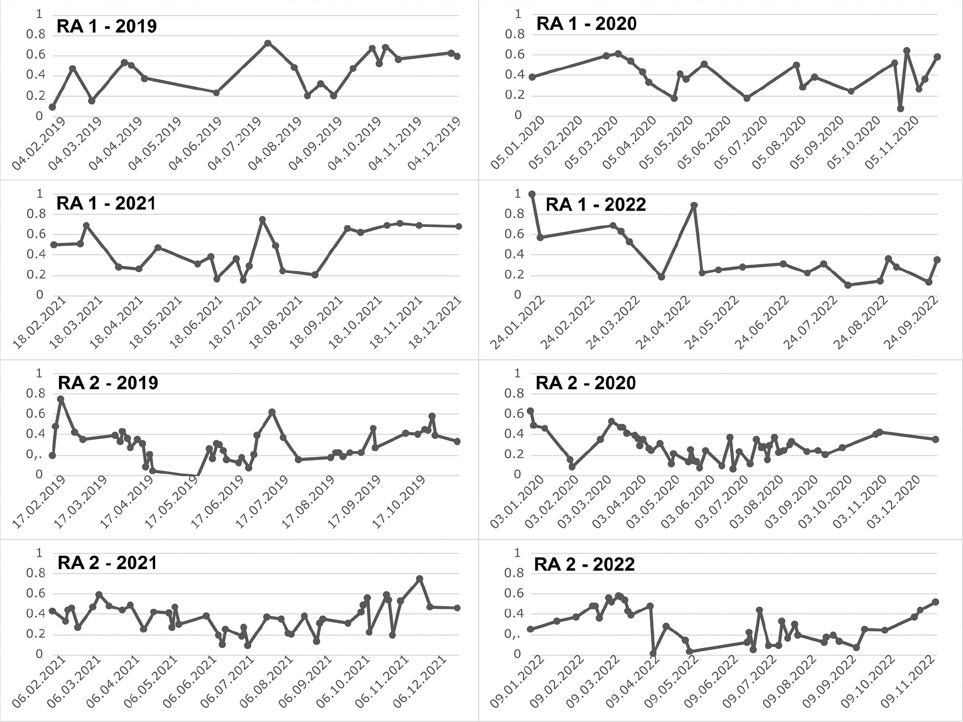
Fig. 19.
Annual NDWI values for Research Area 1 and Research Area 2 within water bodies located in the Vistula River channel for the years 2019–2022. The plots are based on Sentinel-2 scenes with cloud cover below 20% (data source: Copernicus Browser: browser.dataspace.copernicus.eu/). NDWI, normalized difference water index.
This study demonstrated that water indices are highly suitable for conducting comparative analyses over time within large river channels. In all the analysed years, the main channel of the Vistula River was detected with high accuracy. By contrast, the detection of small rivers and water bodies was far less consistent. Their detectability varied significantly between images of the same area acquired under different environmental conditions, making reliable year-to-year comparisons challenging. The nature of the shoreline is crucial for the proper operation of surface water detection procedures. In many cases, temporal changes in the extent of water, particularly in marine or large inland bodies of water, lead to the formation of a broad transition zone, and simply defining the boundary between water and other land cover forms can be problematic (Boak, Turner 2005). This invariably leads to the creation of mixed pixels, whose affiliation to the water zone (threshold problem) must be verified in some way, both manually and using numerical image processing (Ji et al. 2009, Jiang et al. 2014, Astsatryan et al. 2022). Analyses of small streams and water reservoirs are far more sensitive to changes in water level or water colour, often influenced by pollution or the presence of aquatic vegetation, which may reduce their visibility in satellite imagery. These indices can be applied, for example, to monitor changes in river channel morphology, assess the variability of river bars, or detect morphological changes along the shores of larger water bodies. Their usefulness for analysing changes in smaller watercourses, for instance, due to meandering or hydraulic engineering interventions, is more limited. In our study, the transitions between water and vegetation were quite distinct; while wider transition zones were associated with sand bars, due to the dynamics of their formation, they often exposed unvegetated sections. In the case of narrow streams, the final results were influenced by the presence of mixed pixels, which results from the relatively large pixel sizes of the Sentinel-2 image, given the study objectives. There is a risk that narrow features may not be detected due to insufficient spatial resolution, or that detection may not occur consistently across all cases considered in the analysis.
Conclusions
The effectiveness of water body detection was assessed using three spectral indices: NDWI, MNDWI and SWM. The analysis aimed to evaluate the capability of these indices to identify water surfaces within large rivers, small streams and water reservoirs, using two study areas located in the middle Vistula River basin. The obtained results showed very high user accuracy for all analysed indices. This indicates that pixels classified as water almost always corresponded to actual water surfaces. However, producer accuracy was significantly lower, and some water bodies were not identified at all.
The NDWI index demonstrated the highest efficiency and stability in detecting surface waters in the analysed areas. It shows the best performance across all key classification quality metrics, both in numerical and qualitative terms. The SWM index showed moderate but balanced results, with greater variability depending on environmental conditions. Its effectiveness was lower than that of NDWI. The MNDWI index showed the lowest effectiveness, characterised by the lowest producer accuracy and kappa coefficient values. Although its user accuracy remained high, this indicates that it was precise only within the detected pixels, while failing to identify a significant portion of actual water surfaces.
The effectiveness of water detection using spectral indices depends not only on the properties of the indices themselves but also on environmental conditions and satellite image parameters, such as the season in which the imagery was acquired, water level and the presence of pollutants or vegetation that can hinder data interpretation. Spectral indices should be considered a satisfactory method for extracting information from satellite imagery for the analysis of changes in water bodies. A recommended practice is to test several spectral indices on a given image to individually select the one that best reflects the actual environmental conditions.
Acknowledgements
The authors thank the Reviewers for their valuable comments, which certainly helped to improve the quality of this article.
Notes
[1] Contributed by Authors’ contribution
AN: Conceptualisation; Data curation; Methodology; Investigation; Visualisation; Writing – original draft; Writing – review & editing. MF: Conceptualisation; Methodology; Validation; Visualisation; Writing – original draft; Writing – review & editing. KB: Literature review; Methodology; Investigation – analysis of results; Writing – review & editing.