
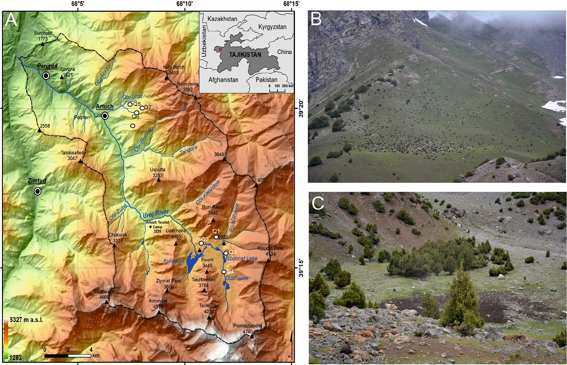
Fig. 1.
A – Study area Q1–Q7 summer livestock camp; B – an example of animal grazing on alpine meadows; C – Qutan in the Fann Mountains – a location in a terrain depression along a watercourse.
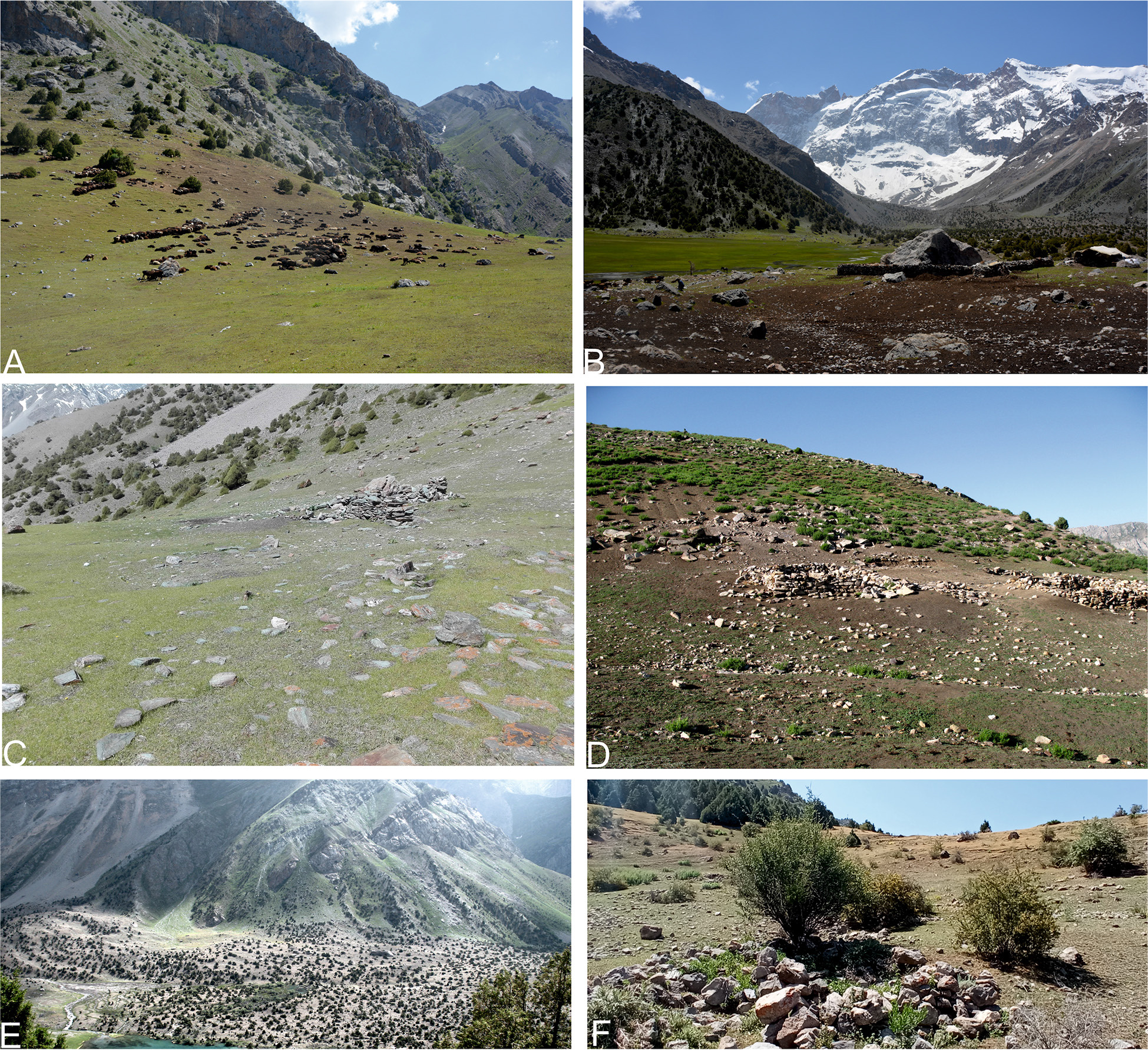
Fig. 2.
Photographs illustrating the study area – qutans in the Fann Mountains: A – Sheep grazing within the qutan Ovulgi Jalol (Q7-OJ) on a slope flattening in the Fann Mountains; B – A fragment of the qutan Murodali Sherali (Q2-MSh) in the headwater zone; C – Ovulgi Alisho sheep qutan (Q1-OA); D – Traces of summer livestock and the breeding of goats and cows during the summer period in Tushqoq (Q6-T); E – Dushacha camp near a water zone (Q4-D); F – Suchti Chuqurak unused cattle camp (Q5-SCh).
Table 1.
Basic characteristics of summer cattle camps.
| Summer cattle camp | Land use | Coordinates | Altitude | Slope | Length of transect | Vegetation |
|---|---|---|---|---|---|---|
| [m a.s.l.] | [°] | [m] | ||||
| Q1-OA | Used | 39°16'22"N 68°12'03"E | 2935 | 9–17 | 35 | Galium aparine, Rumex Paulsenianus, Malva neglecta, Artemisia dracunculus, Convolvulus arvensis, R. Ecae, Berberis oblonga |
| Q2-MSh | Used | 39°16'14"N 68°11'59"E | 2888 | 12–25 | 33 | |
| Q3-B | Used | 39°15'51"N 68°11'42"E | 2913 | 16–19 | 40 | |
| Q4-D | Used | 39°15'02"N 6β°11'50"E | 2954 | 9–12 | 75 | |
| Q5-SCh | Unused since 1989 | 39°20'09"N 68°07'43"E | 2286 | 3–6 | 50 | Artemisia dracunculus, Convolvulus arvensis, Gentiana olivieri, Cichorium intybus, Salvia drobovii, Carex pachystilis, Arum Korolkovii, Plantago lanceolata, P. major, Iris songorica, Eremurusolgae, Ligularia thomsonii, Onosmadi chroanta, Centaurea squarrosa and bushes as Rosa Fedtschenkoana, R. huntica, R. Ecae, Berberis oblonga and Cerasus verrucosa |
| Q6-T | Unused since 2015 | 39°19'38"N 68°08'02"E | 2698 | 8–21 | 35 | |
| Q7-OJ | Used | 39°19'40"N 68°08'32"E | 2851 | 4–19 | 85 | Galium aparine, Rumex Paulsenianus, Malva neglecta, Artemisia dracunculus, Convolvulus arvensis, R. Ecae, Berberis oblonga |
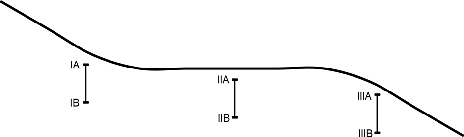
Fig. 3.
Schematic layout of transects and soil sampling sites within the summer livestock camp.
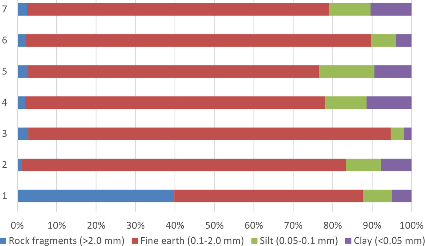
Fig. 4.
Granulometric composition of mineral horizons (Arabic numbers correspond to qutan numbers in Table 1).
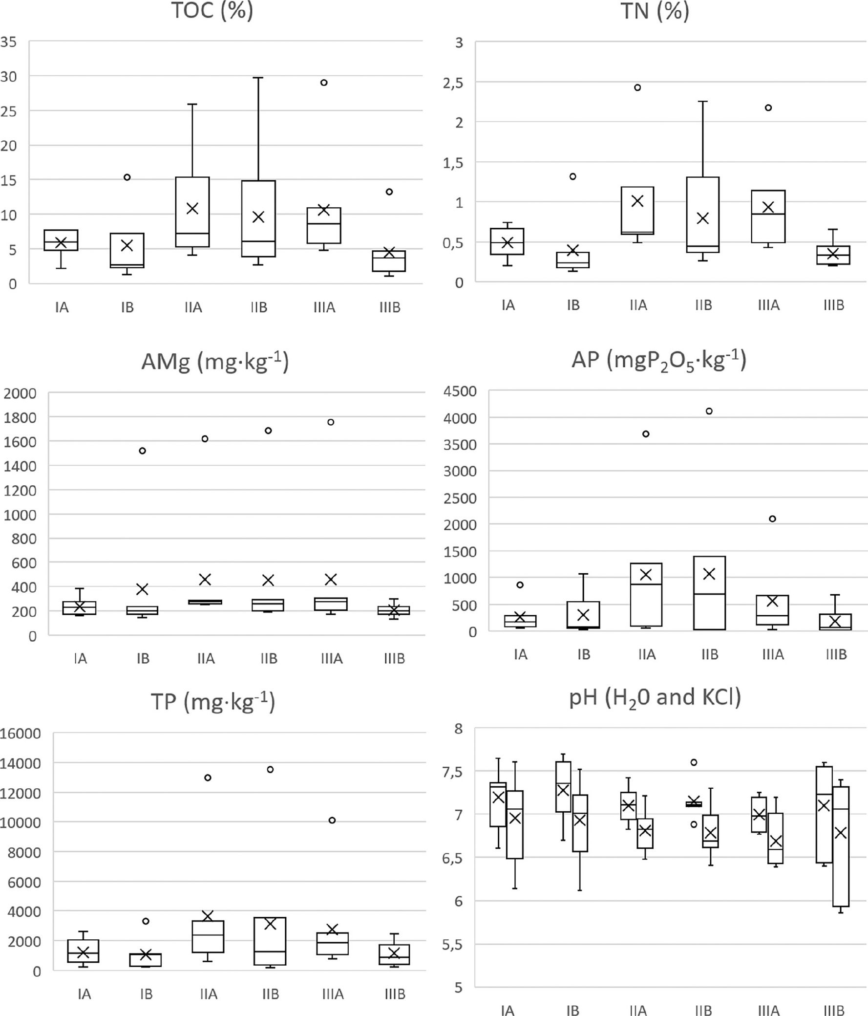
Fig. 5.
Variation of soil properties depending on the sampling location along the transect. Explanations: IA – upper part, upper depth; IB – upper part, lower depth; IIA – middle part, upper depth; IIB – middle part, lower depth; IIIA – lower part, upper depth; IIIB – lower part, lower depth (see Fig. 3). Explanation: The box represents the IQR, the horizontal line inside the box indicates the median, the cross (×) denotes the mean value and whiskers indicate the minimum and maximum values excluding outliers; outliers are shown as individual points.
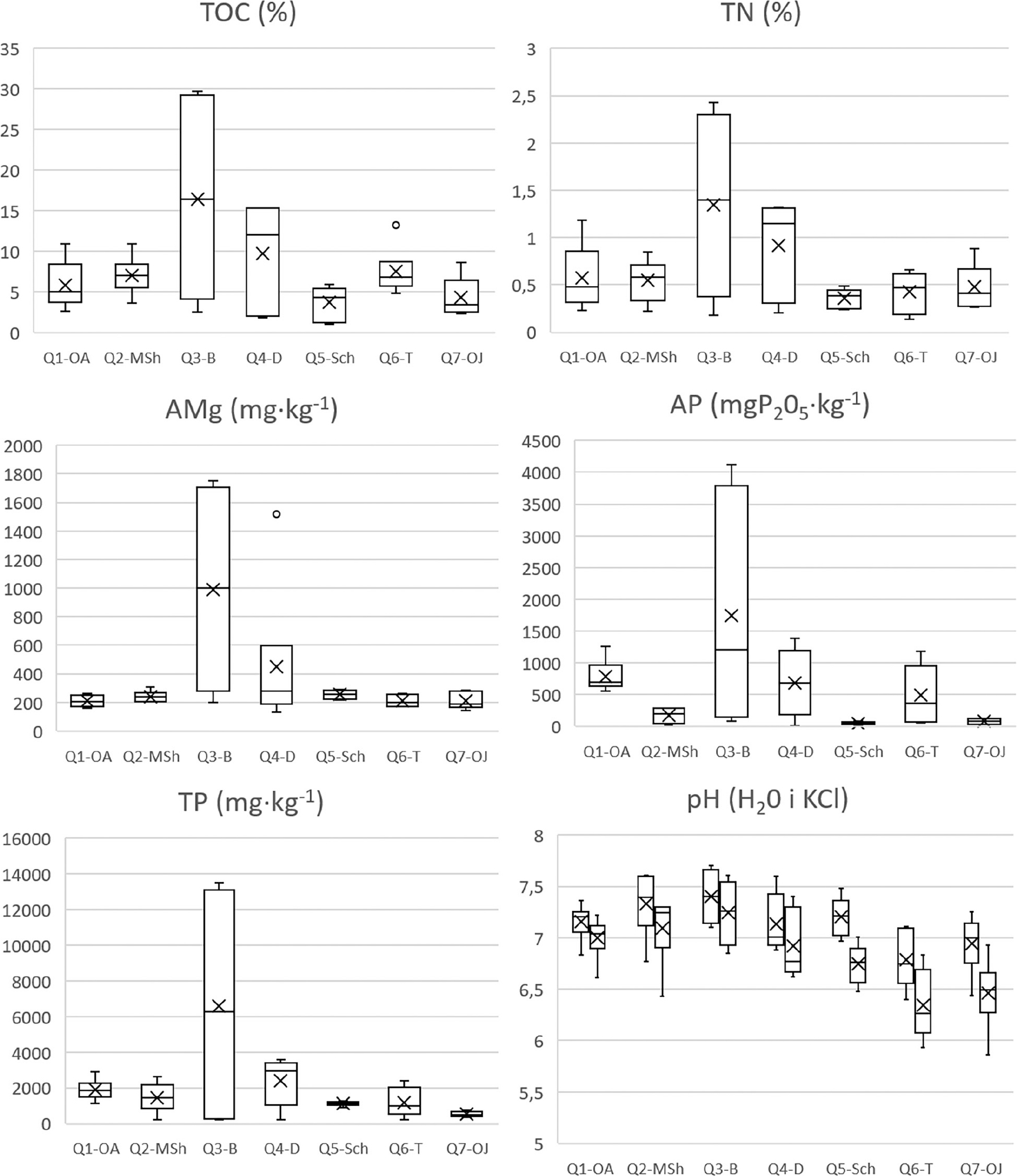
Fig. 6.
Variation of soil properties between individual qutans. Explanations: Q1-OA – Ovulgi Alisho, Q2-MSh – Murodali Sherali, Q3-B – Bibijon, Q4-D – Dushacha, Q5-SCh – Suchti Chuqurak, Q6-T – Tushqoq, Q7-OJ – Ovulgi Jalol (see Fig. 1). Explanation: The box represents the IQR, the horizontal line inside the box indicates the median, the cross (×) denotes the mean value and whiskers indicate the minimum and maximum values excluding outliers; outliers are shown as individual points.
Table 2.
Descriptive statistics grouped by chemical parameters and depth of soil sample collection, along with normality test results.
| Parameter | Depth | Descriptive statistics | CV | W | p | |||||||
|---|---|---|---|---|---|---|---|---|---|---|---|---|
| n | M | Mdn | Min | Max | IQR | SD | SK | |||||
| TN (%) | A | 21 | 0.81 | 0.61 | 0.20 | 2.43 | 0.39 | 0.56 | 1.95 | 0.64 | 0.77 | <0.01 |
| B | 21 | 0.51 | 0.34 | 0.14 | 2.26 | 0.21 | 0.51 | 2.50 | 0.62 | 0.65 | <0.01 | |
| TOC (%) | A | 21 | 9.09 | 6.99 | 2.13 | 29.03 | 3.41 | 6.73 | 2.18 | 0.49 | 0.72 | <0.01 |
| B | 21 | 6.55 | 4.03 | 1.08 | 29.69 | 4.45 | 6.77 | 2.34 | 1.10 | 0.72 | <0.01 | |
| AMg (mg · kg−1) | A | 21 | 385.2 | 263.5 | 160.0 | 1752.5 | 71.0 | 435.4 | 2.91 | 0.27 | 0.46 | <0.01 |
| B | 21 | 346.8 | 214.0 | 132.0 | 1687.5 | 74.0 | 420.9 | 2.93 | 0.35 | 0.45 | <0.01 | |
| AP(mg · P2O5 · kg−1) | A | 21 | 622.8 | 250.7 | 32.7 | 3684.2 | 744.2 | 875.9 | 2.53 | 2.97 | 0.68 | <0.01 |
| B | 21 | 518.1 | 76.3 | 4.4 | 4120.2 | 646.8 | 929.5 | 3.21 | 8.48 | 0.58 | <0.01 | |
| TP (mg · kg−1) | A | 21 | 2540.2 | 1885.0 | 224.8 | 12,980.0 | 1436.0 | 3140.7 | 2.70 | 0.76 | 0.61 | <0.01 |
| B | 21 | 1782.0 | 1112.0 | 201.2 | 13,520.0 | 1343.0 | 2858.6 | 3.79 | 1.21 | 0.52 | <0.01 | |
1 Annotation: n – subgroup size; AP – available phosphorus; CV – coefficient of variation; IQR – interquartile range; M – mean; Max – maximum value; Mdn – median; Min – minimal value; OA – organic-humus; P – p-value; SD – standard deviation; SK – Skewness; TN – total nitrogen; TOC – total organic carbon; TP – total phosphorus; W – Shapiro-Wilk’s test statistics. A – stands for samples originating from the upper soil depth, representing the OA or humus (A) horizons; B – stands for samples collected from lower soil depth, located below the humus layers, mainly from the subsoil B (see Fig. 3).
Table 3.
Results of difference test for upper and lower soil layer.
| Parameter | Unit | Depth | Descriptive statistics | Mann–Whitney test | ||||
|---|---|---|---|---|---|---|---|---|
| M | SD | Average rank | U | Z | p | |||
| Total nitrogen | [%] | A | 0.81 | 0.56 | 27.24 | 100.0 | -3.031 | 0.002 |
| B | 0.51 | 0.51 | 15.76 | |||||
| Total organic carbon | [%] | A | 9.09 | 6.73 | 25.95 | 127.0 | -2.352 | 0.019 |
| B | 6.55 | 6.77 | 17.05 | |||||
| Magnesium | [mg · kg-1] | A | 385.21 | 435.36 | 24.40 | 159.5 | -1.532 | 0.125 |
| B | 346.76 | 420.87 | 18.60 | |||||
| Available phosphorus | [mg · P2 O5 · kg-1] | A | 622.77 | 875.94 | 24.12 | 165.5 | -1.385 | 0.166 |
| B | 518.10 | 929.51 | 18.88 | |||||
| Total phosphorus | [mg · kg−1] | A | 2540.28 | 3140.65 | 24.71 | 153.0 | -1.698 | 0.090 |
| B | 1781.98 | 2858.58 | 18.29 | |||||
1 Annotation: SD – standard deviation; A – stands for samples originating from the upper soil depth, representing the OA or humus (A) horizons; B – stands for samples collected from lower soil depth, located below the humus layers, mainly from the subsoil (B) (see Fig. 3).
Table 4.
Descriptive statistics for six types of soil samples.
| Parameter | Unit | Parameter | IA | IB | IIA | IIB | IIIA | IIIB | Total |
|---|---|---|---|---|---|---|---|---|---|
| Total nitrogen | [%] | M | 0.49 | 0.39 | 1.01 | 0.80 | 0.93 | 0.35 | 0.66 |
| SD | 0.19 | 0.42 | 0.69 | 0.73 | 0.61 | 0.16 | 0.55 | ||
| Min | 0.20 | 0.14 | 0.49 | 0.27 | 0.43 | 0.21 | 0.14 | ||
| Max | 0.74 | 1.32 | 2.43 | 2.26 | 2.18 | 0.66 | 2.43 | ||
| Total organic carbon | M | 5.85 | 5.47 | 10.79 | 9.66 | 10.62 | 4.51 | 7.82 | |
| SD | 1.95 | 4.95 | 7.63 | 9.71 | 8.40 | 4.06 | 6.79 | ||
| Min | 2.13 | 1.22 | 4.08 | 2.64 | 4.80 | 1.08 | 1.08 | ||
| Max | 7.66 | 15.30 | 25.84 | 29.69 | 29.03 | 13.24 | 29.70 | ||
| AMg | [mg · kg−1] | M | 236.7 | 381.0 | 461.3 | 452.1 | 457.64 | 207.2 | 366.0 |
| SD | 76.9 | 502.2 | 508.9 | 546.2 | 573.00 | 53.3 | 423.4 | ||
| Min | 160.0 | 142.0 | 255.0 | 187.0 | 171.0 | 132.0 | 132.0 | ||
| Max | 382.0 | 1517.5 | 1615.0 | 1687.5 | 1752.5 | 301.0 | 1752.5 | ||
| Available phosphorus | [mg · P2O5 · kg−1] | M | 258.9 | 305.4 | 1050.7 | 1065.4 | 558.8 | 183.5 | 570.4 |
| SD | 277.8 | 384.8 | 1261.4 | 1462.4 | 718.6 | 246.0 | 893.6 | ||
| Min | 58.9 | 33.1 | 58.9 | 4.4 | 32.7 | 8.7 | 4.4 | ||
| Max | 858.9 | 1068.2 | 3684.2 | 4120.2 | 2097.2 | 682.3 | 4120.2 | ||
| Total phosphorus | [mg · kg−1] | M | 1224.1 | 1065.6 | 3631.7 | 3138.2 | 2765.0 | 1142.2 | 2161.1 |
| SD | 856.4 | 1081.1 | 4228.0 | 4710.7 | 3286.4 | 810.5 | 2990.8 | ||
| Min | 224.8 | 204.8 | 598.0 | 201.2 | 775.0 | 220.4 | 201.2 | ||
| Max | 2605.0 | 3330.0 | 12,980.0 | 13,520.0 | 10,090.0 | 2455.0 | 13,520.0 |
Table 5.
Results of Kruskal–Wallis test in six samples.
| Sample parameter | Average rank | ||||
|---|---|---|---|---|---|
| Total nitrogen | Total organic carbon | AMg | Available phosphorus | Total phosphorus | |
| [%] | [mg · kg−1] | [mg · P2O5 · kg−1] | [mg · kg−1] | ||
| IA | 21.00 | 21.07 | 18.07 | 20.43 | 19.14 |
| IB | 11.43 | 16.43 | 15.14 | 18.79 | 14.71 |
| IIA | 31.14 | 28.14 | 30.00 | 28.36 | 29.71 |
| IIB | 23.07 | 22.14 | 25.93 | 23.29 | 22.86 |
| IIIA | 29.57 | 28.64 | 25.14 | 23.57 | 25.29 |
| IIIB | 12.79 | 12.57 | 14.71 | 14.57 | 17.29 |
| H Kruskal–Wallis | 15.733 | 9.359 | 9.459 | 5.165 | 7.117 |
| df | 5 | 5 | 5 | 5 | 5 |
| p | 0.008 | 0.096 | 0.092 | 0.396 | 0.212 |
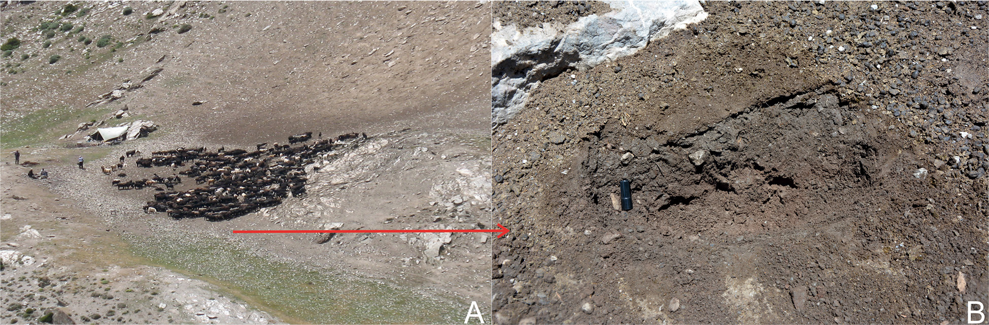
Fig. 7.
Contemporary usable qutan: located on a steep, eroded slope A – and accumulating organic-mineral materials as a result of erosion B.
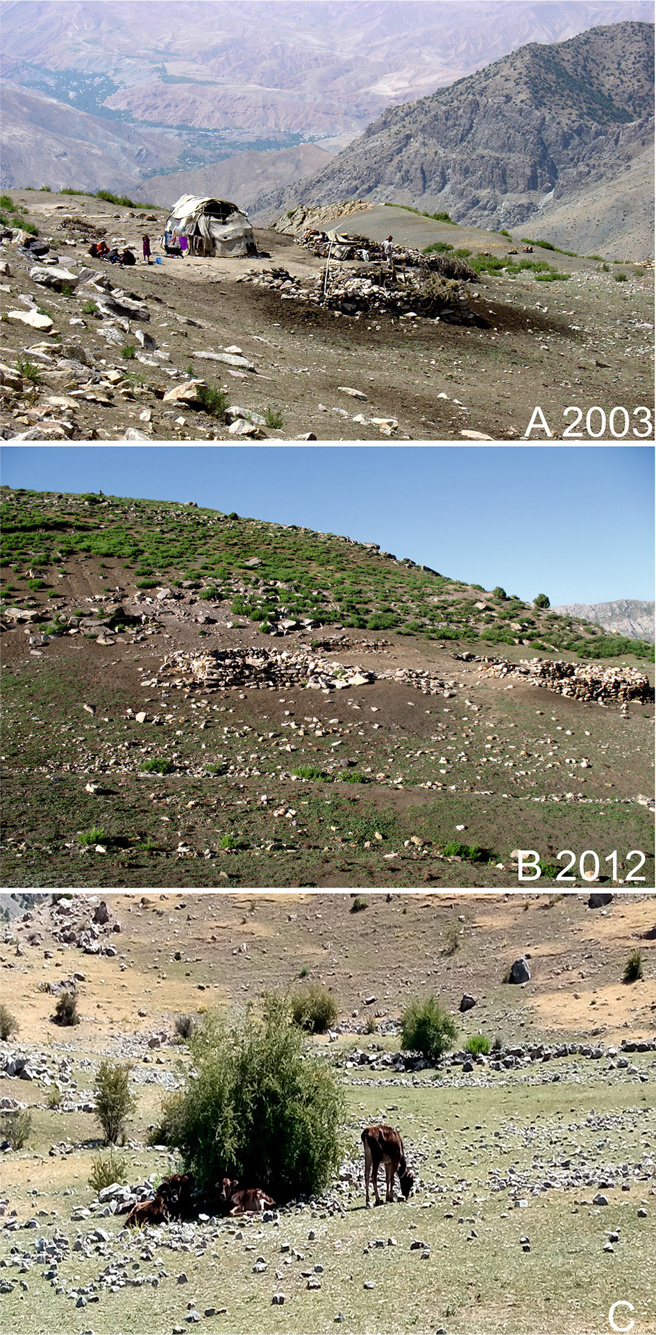
Fig. 8.
Effects of using a summer livestock camp: qutan used in 2003 (A) and not used in 2012 – Tushqoq (Q6-T) (B), with bushes serving as potential resting areas for animals in Suchti Chuqurak (Q5-SCh) (C)