
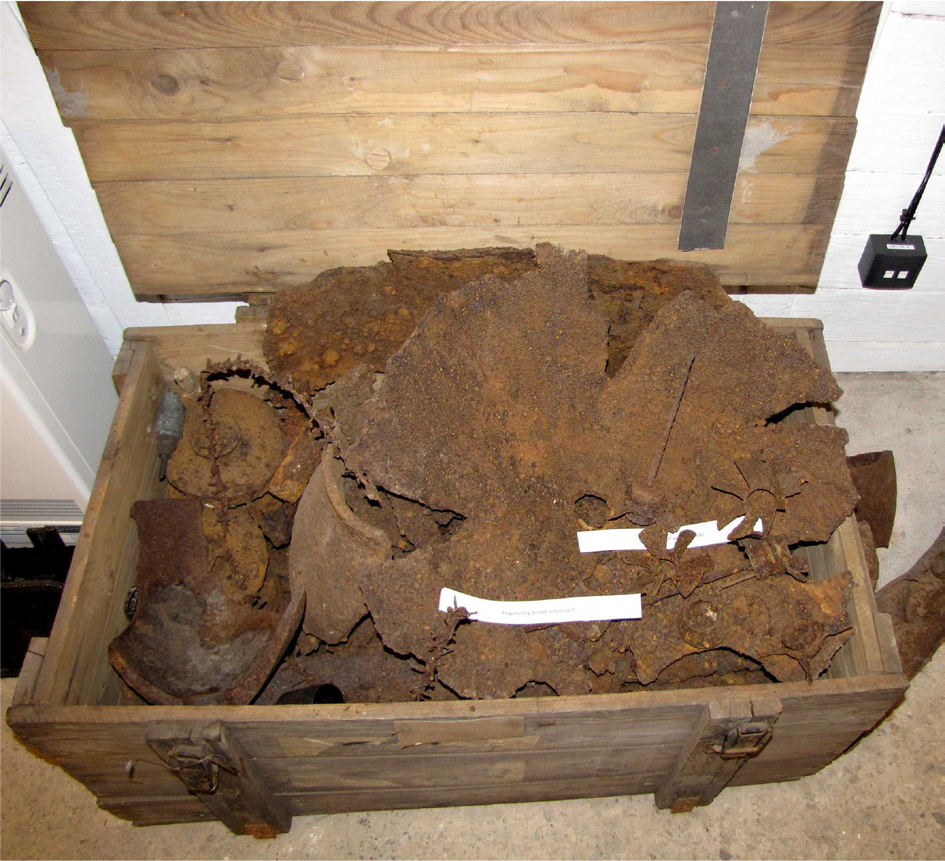
Fig. 1.
Bomb fragments collected from construction site excavations. Exhibits owned by the “Blechhammer 1944” Museum of the Silesian Battle for Fuel in Kędzierzyn-Koźle. (photo: J.M. Waga).
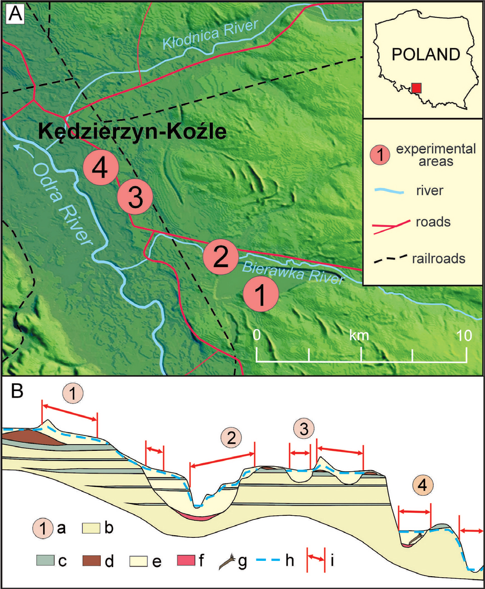
Fig. 2.
A – Location of the study area; B – Synthetic geological cross-section of the study area: a – experimental areas, b – pre-Vistulian sands and gravels, c – massive silts and clays, d – glacial tills with erratic boulders, e – Vistulian sands and gravels, locally organic silts and peats in valleys, f – boulder horizon, locally with erratic boulders, g – “black oaks”, h – water table, i – zones prone to UXB risks.
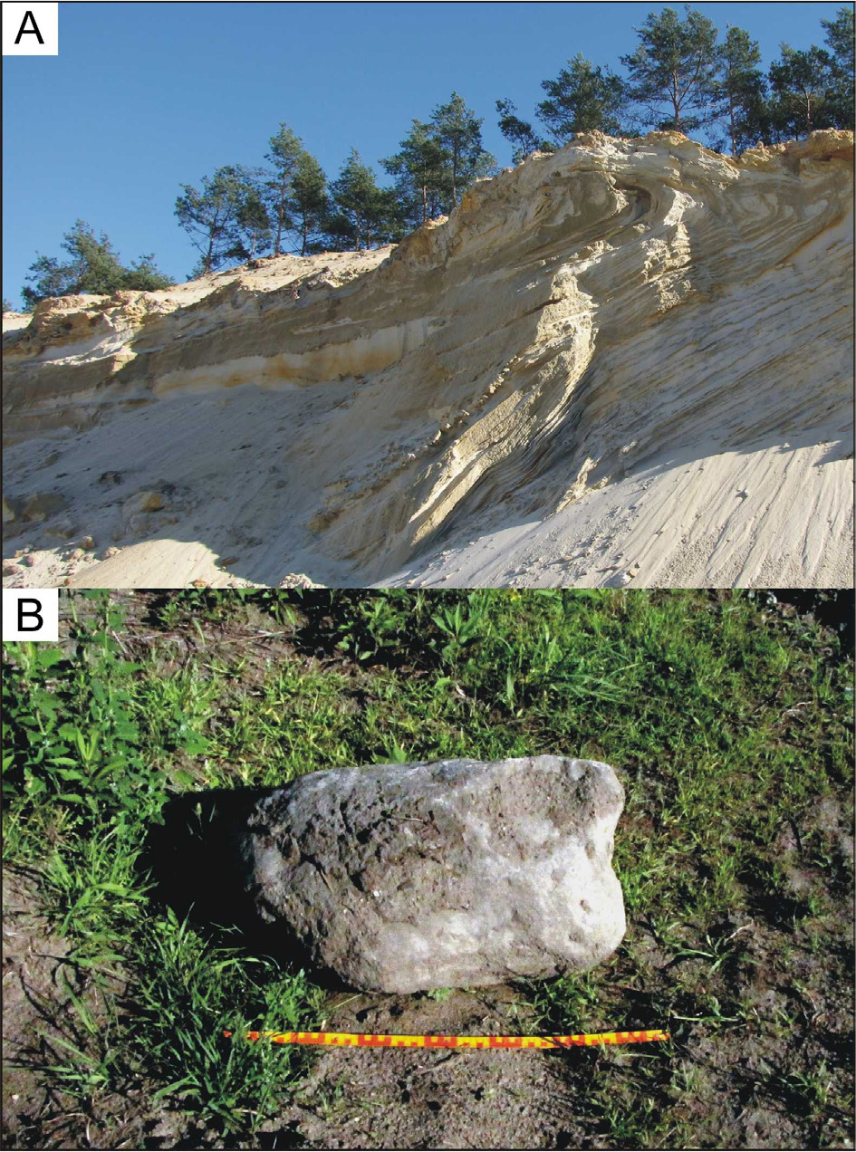
Fig. 3.
A – Glacitectonically disturbed series of marginal sediments with massive silts at experimental area 1; B – Erratic boulder resting on silt, removed from a shallow excavation in experimental area 3 (photo: J.M. Waga).
Table 1.
Methods and equipment used in the study.
| Abbrev. | Technology | Device | Manufacturer | Depth (m) |
|---|---|---|---|---|
| MAD | Magnetic anomaly detection | Pioneer VLF | Bounty Hunter | 0–0.65 |
| PM | Proton magnetometry | Maggie magnetometer | Schonstedt | 0–5.5 |
| ECM1 | Electromagnetic conductivity | EM31-MK2 meter | Geonics | 0–6.0 |
| ECM2 | Electromagnetic conductivity | CMD Explorer meter | GF Instruments | 0–6.7 |
| GPR | Ground penetration radar | Pro Ex RAMAC X3M | MALÅ | 0–4.8 or 0–11.5 (recording range 97.94 or 229.62 ns depending on the antenna used) |
| ER | Electrical resistivity | ABEM Terrameter SAS 4000 with ABEM LUND Imaging System | ABEM Instrument | 0–7.2 or 0–14.4 (recording range depending on the electrode spacing: 1 or 2 m) |
Table 2.
Areas and lengths of the profiles investigated by different geophysical methods.
| Experimental areas | MAD [m2] | PM [m2] | ECM1 [m2 or *m] | ECM2 [m2] | GPR [m] | ER [m] |
|---|---|---|---|---|---|---|
| 1a | 3800 | 3800 | 600 | 800 | – | – |
| 2a | 10000 | 10000 | 400 | – | 1120 | 80 |
| 3a | 3150 | 3150 | 240 | – | 290 | 40 |
| 3b | 2250 | 2250 | – | – | 370 | – |
| 3c | 12000 | 12000 | *40 | – | 370 | – |
| 3d | 4300 | 4300 | 960 | – | – | – |
| 4a | 1500 | 1500 | *52 | – | – | – |
| 4b | 1800 | 1800 | *74 | – | – | – |
| 4c | 3050 | 3050 | *69 | – | – | – |
| 4d | 950 | 950 | *65 | – | – | – |
| 4e | 2200 | 2200 | – | – | – | – |
| Total | 45000 | 45000 | 2200 + *300 | 800 | 2150 | 120 |
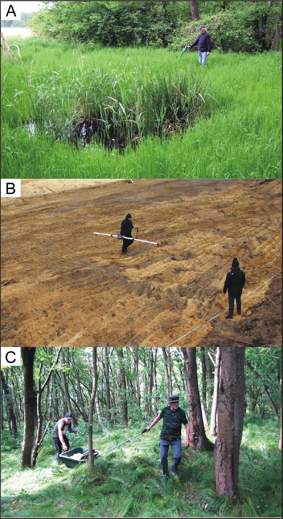
Fig. 4.
A – Ground scanning with a proton magnetometer in the vicinity of a flooded UXB intake crater (in the foreground); B – Ground scanning with a Geonics EM31-MK2 conductivity meter; C – Ground profiling in difficult forest terrain using the Mala RAMAC X3M GPR (photo: J.M. Waga).
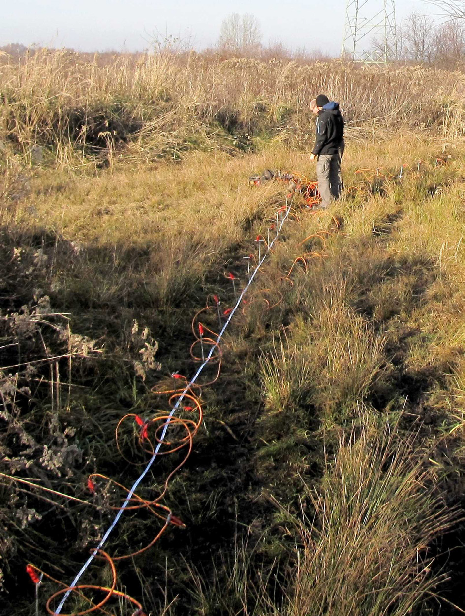
Fig. 5.
Electrical resistivity tomography using ABEM’s LUND Imaging System (photo: J.M. Waga).
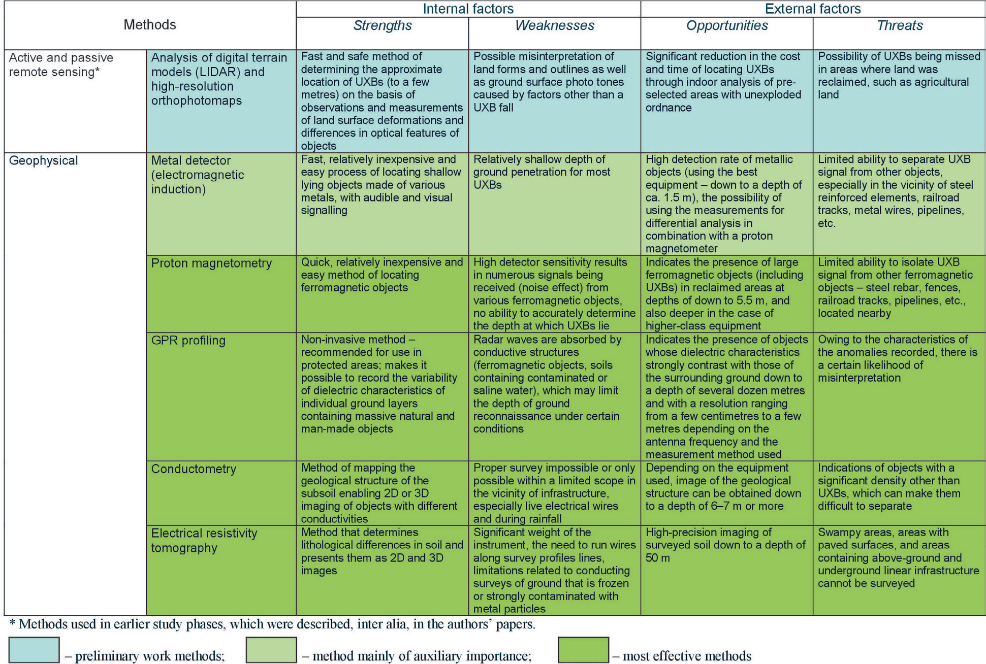
Fig. 6.
Characteristics of methods used to locate UXBs (in SWOT terms).
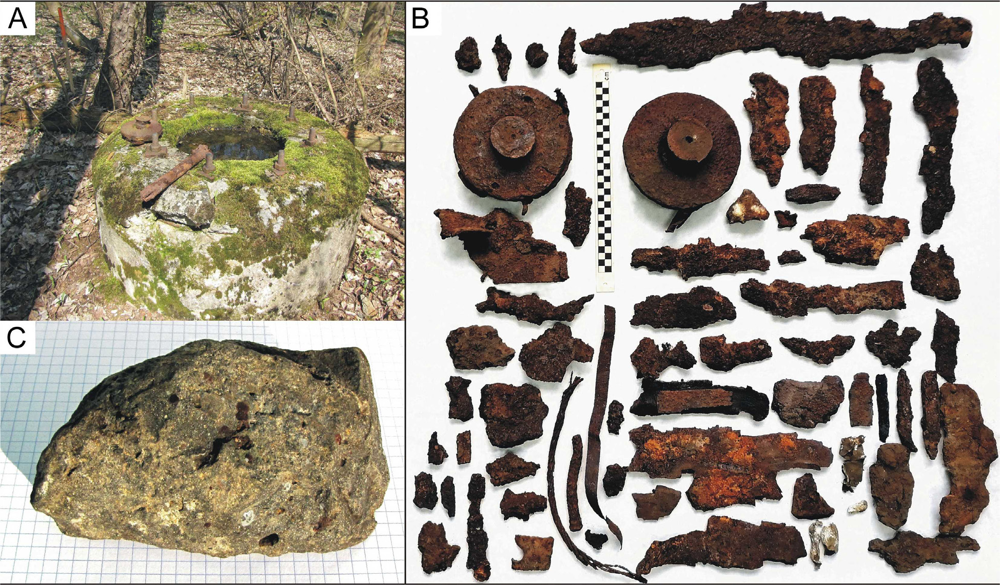
Fig. 7.
Examples of surface finds identified using the proton magnetometer: A – tail base plug of 500 lb bomb with tail fuse fragments and a peg made of steel pipe lying on the concrete base of a 75mm Flak 97 gun that was part of Schwere Heimat-Flak-Batterie 212/VIII Alt Cosel; next to those, an orange stake marking a future development project (photo: J.M. Waga); B – fragments of bombs, of a power line and possibly of a B-24 plane (photo: B. Szypuła); C – Rock fragment with ferromagnetic properties (photo: J.M. Waga).
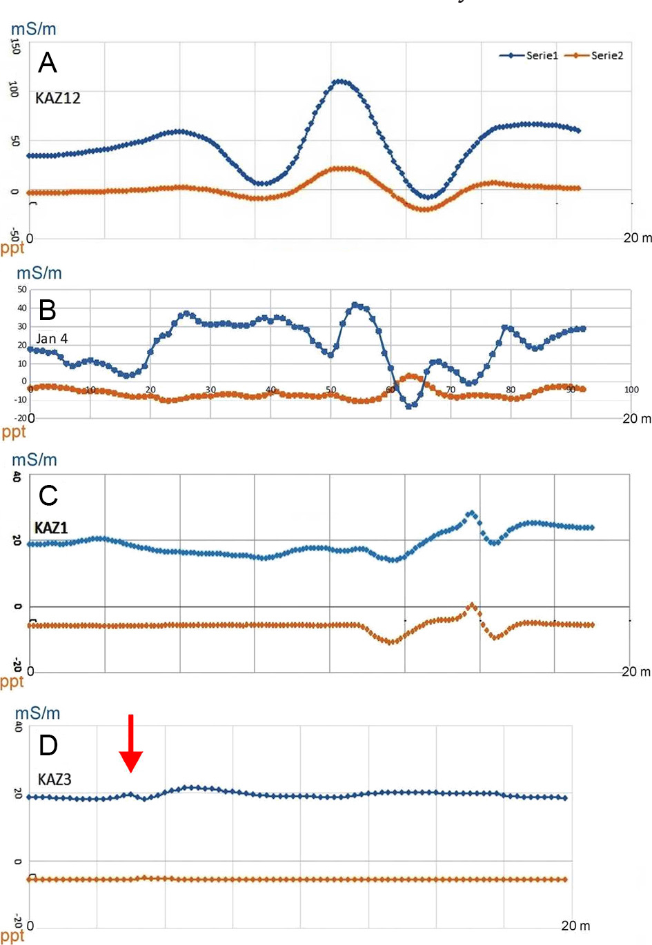
Fig. 8.
Conductivity profiles from measurements performed using the Geonics EM31-MK2 instrument. Serie 1 – apparent conductivity, Series 2 – magnetic component – in-phase. Anomalies indicating: A – the presence of a steel pipe from a former water pipeline; B – presence of shrapnels in a buried crater after a detonated bomb; C – the potential presence of UXB; D – likely drift channel trace (anomaly indicated by a red arrow) located between the UXB inlet crater and its location.
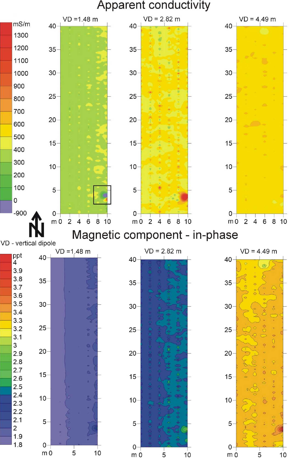
Fig. 9.
Layered map generated from CMD-Explorer conductivity meter readings with a potential UXB identified (location marked with a square).
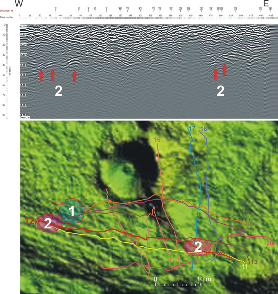
Fig. 10.
GPR profiling in a forest area: 1 – UXB fall site remodeled by later earthworks, 2 – subsurface object zones, 11-20 – profile lines.
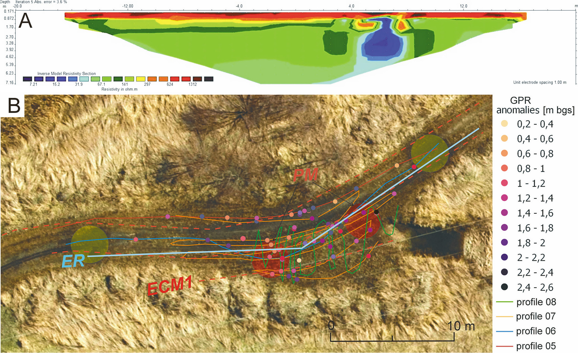
Fig. 11.
Experimental area 3: A – diagram presenting electrical resistivity tomography results obtained in a wetland; B – profiles lines ECM1, GPR, ER and two concentrations of PM signal occurrence (red circles). Large yellow circles – probable remnants of the UXB fall. The profile described as ECM1 is shown in Fig. 8B.
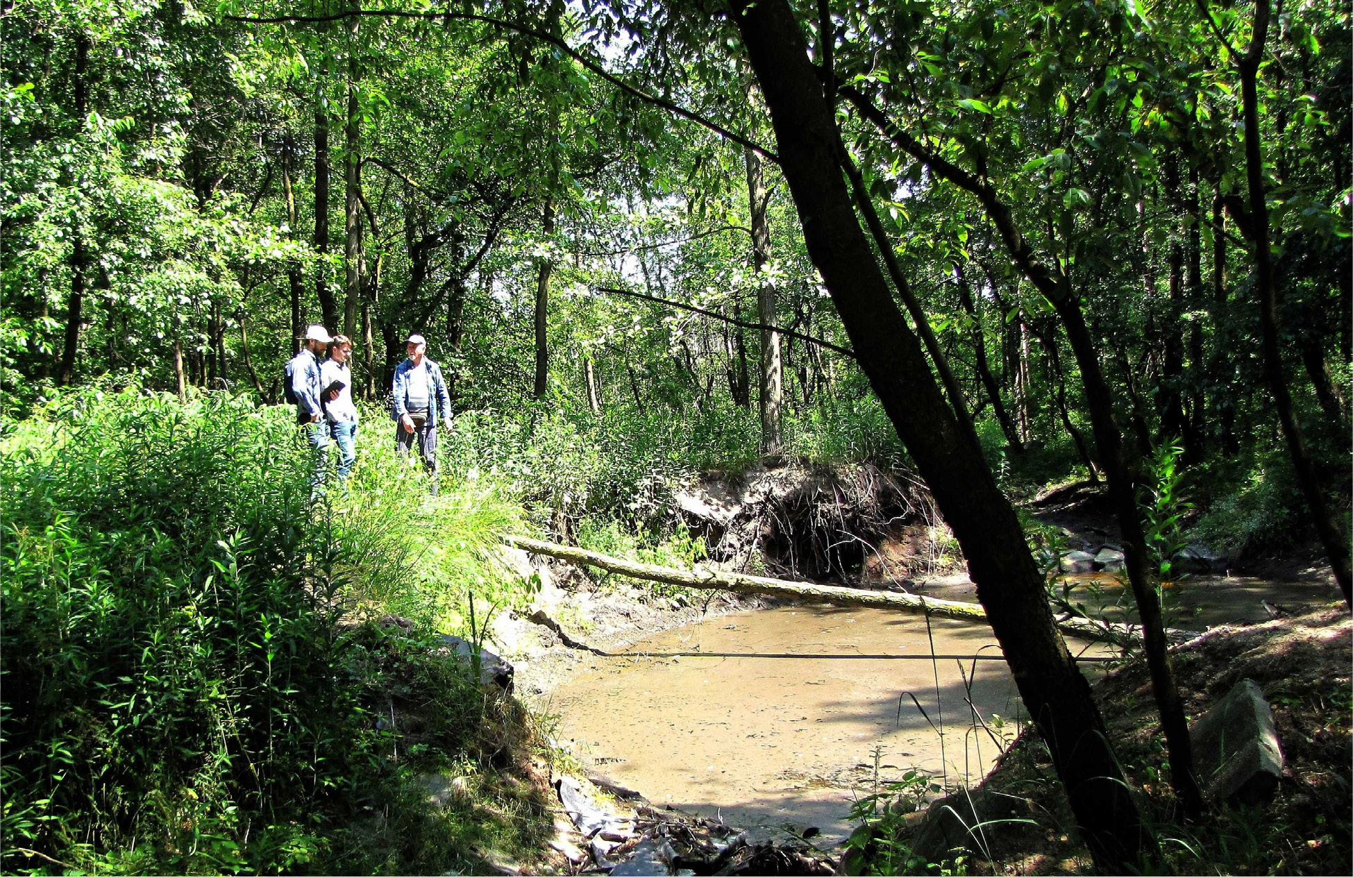
Fig. 12.
Authors in the vicinity of a crater formed as a result of a spontaneous UXB explosion in late 2021/early 2022 (photo: J.M. Waga).