Glacial curvilineations (GCLs) are subtle, elongated ridge landforms occurring typically in swarms within tunnel valleys and interpreted as the erosional imprint of subglacial meltwater activity. Lesemann et al. (2010, 2014) systematically defined them first; these features have since been recognised across the southern margin of the Last Scandinavian Ice Sheet (Adamczyk et al. 2022), yet their identification remains challenging due to their low relief and morphological complexity. Despite advances in high-resolution digital elevation models (DEMs), delineating GCLs with consistency remains a predominantly manual task, reliant on geomorphologist expertise and terrain-reading intuition. Their formation mechanisms, spatial organisation and potential role in subglacial drainage networks make GCLs important indicators of past ice-sheet dynamics. Their elusive nature mirrors the hidden, dynamic forces that once shaped the ice-sheet bed.
In recent years, geomorphometric methods have enabled the automation of landform classification, offering scalable alternatives to visual interpretation. Among these, geomorphons (Jasiewicz, Stepinski 2013) and the Topographic Position Index (TPI, Weiss 2001) have emerged as commonly applied techniques for detecting local terrain forms. However, the extent to which these methods can accurately detect and characterise GCLs – landforms defined as much by spatial coherence as by form – is not well understood. The present study addresses this gap by comparing automated outputs from geomorphons and TPI against a manually refined reference dataset of GCLs in the Drawsko Lakeland, northwestern Poland. The Drawsko Lakeland provides an ideal setting for this analysis, as it hosts well-preserved GCL fields that have been previously analysed using manual approaches.
GCLs are elongated, sinuous and parallel ridges separated by shallow depressions (troughs), typically less than 10 m in height and extending for several kilometres (Hermanowski, Piotrowski 2023). These features occur in swarms composed of morphologically coherent ridges and are predominantly found within subglacial tunnel valleys, where they form distinctive ridge assemblages. Initially, GCLs were formally defined as a unique category of subglacial landform by Lesemann et al. (2010, 2014), based on observations from the Dobrzyń Plateau in Poland. Prior to this, similar forms had been recognised but interpreted in different ways as drumlins, eskers, or push moraines (Jewtuchowicz 1956, Lamparski 1972, Ber 1986, Wysota 1994, Olszewski 1997, Lewandowski et al. 2003, 2006).
Subsequent studies have documented GCLs in Poland, Germany and Denmark (Adamczyk et al. 2016, 2022, Weckwerth et al. 2019, Adamczewska 2023, Hermanowski, Piotrowski 2023, Wysota et al. 2024), expanding the geographic scope in North America (Clark, Livingstone 2018). The most comprehensive inventory to date is provided by Adamczyk et al. (2022), who mapped 59 GCL fields across the southern margin of the Last Scandinavian Ice Sheet. Detailed morphometric analyses were conducted for 43 of these fields, encompassing a total of 137 swarms. Their classification, grounded in landform arrangement and tunnel valley morphology, has significantly advanced understanding of GCL distribution and internal variability. However, it should be noted that their analyses were based solely on surface morphology derived from high-resolution Light Detection and Ranging (LiDAR) DEMs, without accompanying sedimentological or geophysical validation.
Several studies have contributed to the ongoing refinement of GCL interpretation. Lesemann et al. (2010) introduced the term and proposed an erosional origin linked to subglacial meltwater vortices. This interpretation was further supported by sedimentological and geophysical investigations, including resistivity tomography, in Lesemann et al. (2014). Adamczyk et al. (2016) examined the Zbójno field and emphasised postglacial infilling processes within inter-ridge troughs. Weckwerth et al. (2019, 2024) and Wysota et al. (2024) associated GCL development with subglacial routing of Late Weichselian outburst floods, identifying both large-scale and fine-grained erosional features. Hermanowski and Piotrowski (2023), working in the Stargard drumlin field, presented sedimentological evidence that GCLs are sculpted from underlying till, reinforcing the erosional model. By contrast, Clark and Livingstone (2018) proposed a divergent hypothesis, stating that GCLs formed through subglacial slope and bank failure near tunnel valleys and subglacial lakes – an interpretation derived solely from morphometric DEM analysis, without lithological data. Finally, Adamczewska (2023) applied geomorphometric analysis to curvilinear ridges in the Drawsko Lakeland, using LiDAR-based DEMs to characterise their spatial structure and topographic properties. The growing body of DEM-derived morphometric data underscores the potential of automated or semi-automated terrain analysis methods in studying GCLs. This study aims to evaluate the extent to which such approaches can effectively delineate and characterise these subtle glacial features, and how closely they approximate manual interpretation.
With the rapid development of information technologies and computational systems, geomorphometry has gained new analytical capacities that enable more precise modelling and interpretation of Earth surface forms. Contemporary geomorphometry is grounded in digital elevation data, using numerical methods to extract and visualise detailed terrain features. DEMs and surface analysis algorithms now form the backbone of geomorphological research, thus allowing for the quantitative characterisation and classification of landforms through automated tools (Gawrysiak 2018).
Today, numerous automated landform classification methods rely on metrics derived from DEMs, employing algorithms that identify characteristic surface features such as ridges, valleys and slope breaks. Jasiewicz and Stepinski (2013) observed that most of these methods are based on principles of differential geometry and differ primarily in their use of geomorphometric variables and the scale or type of spatial units they classify. Broadly, they can be categorised into cell-based and object-based approaches (cf. Dragut, Blaschke 2006, 2008, van Asselen, Seijmonsbergen 2006, Ghosh et al. 2009).
Among the simpler yet widely applied terrain metrics is the TPI, which compares the elevation of each cell to the mean elevation of a defined neighbourhood. Weiss (2001) initially proposed TPI as a simplification of the earlier Landscape Position Index (Fels, Zobel 1995), it has since become common in geomorphological mapping and habitat modelling. Its implementation in Geographic Information System (GIS) platforms – most notably through the ArcGIS extension developed by Jenness (2006) – requires only a raster-based elevation input, making it computationally accessible and broadly applicable.
The introduction of gridded elevation models (Miller, Laflamme 1958) marked a pivotal shift in geomorphological analysis, enabling algorithmic classification approaches based on surface derivatives (Evans 1972, Krcho 1973). These early methods accelerated the quantification of land surface features, which had previously been derived manually from topographic maps (Żynda 1976). However, traditional schemes based on local derivatives have not always aligned with human cognitive perceptions of landforms (Jasiewicz, Stepinski 2013). In response, Jasiewicz and Stepinski introduced the geomorphon approach – a machine vision method that bypasses derivative calculations and instead classifies terrain using a ternary pattern of relative elevation in eight directions. This method assigns each cell to 1 of 10 elementary landform types. Geomorphons have since been applied to terrain analysis in various morphogenetic zones across Poland (Gawrysiak 2018, Jancewicz et al. 2022, Gawrysiak, Kociuba 2023).
Young glacial landscapes such as those of the North European Plain pose particular challenges for derivative-based morphometric classification (see Dyba, Jasiewicz 2022). These terrains are often morphologically immature and complex, composed of forms that resist simple geometric categorisation and are better described through genetic typologies (e.g. moraines, outwash plains, tunnel valleys). Accordingly, the development of automated classification methods can bridge the gap between elementary shape recognition and geomorphogenetic interpretation. In this context, the present study assesses the potential of the geomorphon approach (Jasiewicz, Stepinski 2013) to support the classification of genetically meaningful landforms within the postglacial landscapes of the Polish Lowlands. Specifically, it evaluates how effectively this method can detect and characterise subtle, spatially coherent features such as GCLs. To date, no study has systematically compared the performance of geomorphons and TPI in identifying GCLs; this work is a pioneer one benchmarking both methods against a manually refined reference dataset.
This study aims to assess the reliability and interpretative fidelity of automated GCL mapping techniques by comparing morphometric outputs derived from geomorphons and TPI-based analyses with a manually refined reference dataset. Working within a postglacial setting, the study investigates the ability of these methods to delineate and characterise GCL landforms and explores their potential to facilitate semi-automated classification of genetically distinct forms in young glacial terrains. Quantitative indicators, such as area coverage, feature count and elevation parameters, are used to evaluate method performance relative to the manual baseline.
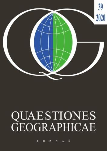
The study area is located in northwestern Poland, within the mesoregions of Drawsko Lakeland and Szczecinek Lakeland (Solon et al. 2018, Richling et al. 2021). Field investigations focussed on the Komorze tunnel valley, a marginal glacial trough trending W–E to WNW–ESE, which has a chain of lakes including Wilczkowo, Drawsko, Żerdno and Komorze (Fig. 1). This valley forms part of a broader ice-marginal landscape, extending over 40 km and reflecting complex interactions between glacial advance, stagnation and meltwater dynamics during the Late Weichselian (Marsz 1973).
Location of the study area in the Drawsko Lakeland, showing the Komorze tunnel valley and surrounding mesoregions.
The region lies on the southern slope of a postglacial ridge system, shaped by the advance and frontal-areal deglaciation of the Pomeranian Phase of the Weichselian Glaciation, dated to approximately 17–16 ka (Marks 2012, Tylmann et al. 2019). The landscape is typical of young glacial terrain, featuring a mosaic of undulating, hilly and flat landforms of glacial and glaciofluvial origin, interspersed with kame hills, kettle depressions and morainic plateaus. Elevations range from over 220 m a.s.l. to approximately 50 m a.s.l. in valley floors, with relative relief reaching up to 173 m. Steeper slopes (10–30°) are associated with kame-and-dead-ice topography, tunnel valleys and marginal escarpments, while vast terrain exhibits low gradients (0–2°) (Karczewski 1989, Lewandowski et al. 2006, Mazurek et al. 2024).
Local geomorphology reflects a complex subsurface architecture resulting from multiple glacial-interglacial cycles. Within this framework, buried subglacial valleys commonly exploit pre-Quaternary tectonic lineaments, particularly those trending SE–NW (Dobracka, Piotrowski 2002). It should be noted that there is a deep, east–west oriented fluvial valley, probably formed during the Holsteinian and Eemian Interglacials, which corresponds with the present-day alignment of the Pile–Komorze–Żerdno lake system. Its orientation and persistence suggest structural control by reactivated tectonic depressions and the influence of subaerial drainage systems active during interglacial periods and modification by overriding ice masses (Marsz 1973, Lewandowski et al. 2006).
In the study area, deposits from multiple glaciations are present, including those attributed to the Nidanian (MIS 22), Sanian I (MIS 16), Sanian II (MIS 12), Odranian (MIS 6), Wartanian and Weichselian (MIS 2) stages. North of the Pomeranian Phase marginal zone (Fig. 1) is a series of morainic plateaus (70–110 m a.s.l.) composed of ablation tills rich in boulders, with gravel and sand often occurring at hilltops. Kame hills and melt-out depressions are widespread, reflecting stagnation and ice melt during deglaciation. Foreland sandur plains, formed in two principal levels, are associated with the activity of meltwaters flowing southward from the ice margin (Karczewski 1997, Mojski 2005).
Hydrologically, the area is characterised by narrow, deep ribbon lakes of subglacial origin, predominantly aligned along NNW–SSE and ENE–WSW axes. These lakes typically have steep shores and feature submerged basins and shoals. The largest, Lake Drawsko, covers 17.97 km2 and reaches a depth of 82.2 m. Lake Komorze, the central feature of the tunnel valley under study, spans 3.89 km2 and reaches a maximum depth of 34.3 m (Map of Hydrographic Division of Poland, 2004). The alignment of the Komorze trough corresponds with a buried tunnel valley and marks the maximum extent of the Pomeranian ice sheet (Dobracka, Lewandowski 2002, Lewandowski et al. 2003).
GCLs in the Komorze through were described by Adamczyk et al. (2022), who classified the Łubowo site – referred to in the present study as the Komorze tunnel valley – as a compound tunnel valley containing several swarms of GCLs. These features were further examined by Adamczewska (2023), who conducted geomorphometric analyses using high-resolution LiDAR data. Her study emphasised the spatial coherence and morphological regularity of the curvilinear ridges within the young glacial landscape of the Drawsko Lakeland. Together, these works underscore the geomorphological significance of the Łubowo field as a representative site for studying subglacial meltwater-driven erosion processes.
The primary source data for this study consists of a DEM derived from airborne LiDAR data provided by Head Office of Geodesy and Cartography in Poland (GUGIK,geoportal.gov.pl). The original DEM, with a resolution of 1 m, offers high precision for geomorphometric analysis. However, such high-resolution data may accentuate minor microrelief features that are not relevant for broader-scale interpretations, particularly in the context of identifying GCLs. To evaluate the optimal resolution for GCL detection, the DEM was resampled to 5-m and 10-m grids. This resampling aimed to balance terrain detail with interpretability at broader spatial scales, enabling a more effective extraction of morphometric patterns.
All spatial analyses, including manual digitisation, geomorphometric attribute computation and postprocessing, were conducted using SAGA GIS 9.5.1 and ArcGIS Pro 3.2.0. Rasterbased analyses were conducted primarily in SAGA GIS, while vector editing, statistical assessment and visualisation were performed in ArcGIS Pro. Primary terrain attributes included slope, aspect, curvature and hillshade, which facilitated both visual interpretation and manual delineation. Two secondary attributes – TPI and geomorphons – were selected for automated classification and are described in detail below.
Individual GCLs were manually delineated based on the 5-m DEM, supported by a shaded relief using a standard illumination azimuth of 315°. While this lighting direction enhances general topographic visibility, it may introduce directional bias. To minimise this effect, additional geomorphometric parameters (e.g. slope, curvature) and visual verification with orthophotomaps were used to support feature identification. The analysis focussed on the Komorze tunnel valley, where representative ridge forms were digitised and grouped into five swarms of GCLs. The swarms were delineated based on the alignment of ridge crests and the intervening depressions, with particular attention to length, width and consistent axial orientation among ridges. These manually delineated swarms served as spatial reference units for subsequent morphometric and comparative evaluation. The manual delineation represents an expert-guided interpretation of the ridge morphology and functions as a baseline for assessing the reliability of automated methods.
The TPI calculates the difference between the elevation of a focal cell and the average elevation of its surrounding neighbourhood (Weiss 2001). Positive TPI values identify cells raised or elevated above their surroundings (e.g. ridges or hilltops), while negative values correspond to depressions such as troughs, valleys or hollows. The sensitivity of TPI to landform scale is influenced by the size of the neighbourhood: larger windows emphasise broader forms while smaller windows capture finer features (De Reu et al. 2013). TPI was computed using square neighbourhoods of 50, 100, 150 and 200 m for the 1 m DEM, and 10, 25, 50, 75 and 100 m for the resampled 5 m and 10 m DEMs. The 5 m DEM, combined with neighbourhood sizes of 50, 75 and 100 m, yielded the most interpretable results and was therefore selected for further analysis. TPI layers were reclassified into four intervals (TPI >0.5, >1, >1.5 and >2), and visual comparison with hypsometry indicated that TPI >1 was optimal for delineating GCL ridges.
Geomorphons, introduced by Jasiewicz and Stepinski (2013), classify terrain into 1 of 10 elementary landform units (e.g. ridge, valley, flat) based on local elevation contrasts assessed in eight cardinal directions. Each unit is derived from a ternary 8-tuple pattern that captures the relative height of a cell and its surrounding neighbourhood. For this study, ridge-related classes (ridge, shoulder, peak, spur) were aggregated to identify potential GCL ridges. Two key parameters, lookup distance and flatness threshold (FT), control geomorphon sensitivity. Lookup distances of 100 and 500 and FTs from 1 to 5 were tested. After visual and hypsometric comparison, optimal settings were determined with a lookup distance of 100 and FTs of 1, 2 and 3.
For each method – manual, TPI-based and geomorphon-based – basic morphometric metrics were calculated, including the area, length and elevation (maximum, mean and minimum) of each identified landform. At the swarm level, additional parameters such as total swarm area, total GCL area and its proportional coverage of the swarm, average GCL width and total number of GCLs were computed. All calculations of morphometric attributes were performed in the EPSG:2180 (PUWG 1992) projected coordinate system, which is suitable for preserving distances and areas in the Polish territory.
Limitations inherent in automated classifications are addressed through postprocessing steps, which remove internal gaps, exclude polygons smaller than 1000 m2 and clip outputs to predefined swarm boundaries.
The core of this study lies in the comparison of morphometric outputs derived from automated methods (TPI and geomorphons) to those from manual interpretation. Quantitative metrics such as form count, area, percent swarm coverage and elevation parameters were summarised per method and swarm. Boxplots were generated in RStudio to visualise differences and distributional tendencies across methods.
For evaluating the fidelity of each method, percentage differences between automated outputs and the manual baseline were calculated and visualised using a heatmap. This map illustrates the direction and magnitude of deviation across morphometric metrics, offering a nuanced assessment of each method’s capacity to replicate the morphometric footprint of GCLs. The visualisation was generated in Google Colab using Python libraries.
This integrated approach represents the first structured comparison of geomorphon- and TPI-based GCL delineation methods against a manually validated benchmark. It contributes greatly to the effort of assessing automated classification reliability in postglacial terrain and in enhancing scalable methods for identifying subtle, genetically meaningful landforms.
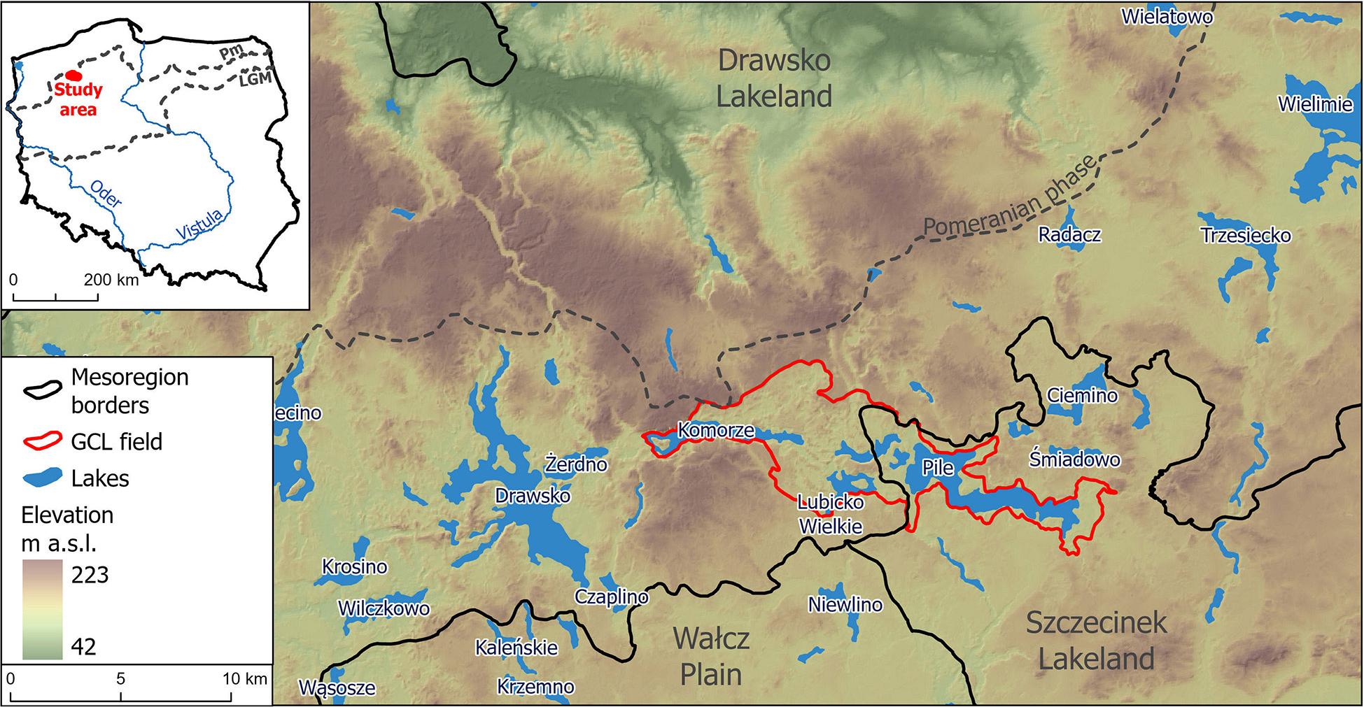
The Komorze tunnel valley exhibits a latitudinal orientation and covers a total area of 58.18 km2. Analysis of the DEM revealed that within this valley, absolute elevations are in the range of approximately 134 m a.s.l. to over 157 m a.s.l. GCLs are clearly visible within the valley as sinuous, parallel ridges forming swarms of morphologically coherent features. Five distinct GCL swarms were delineated – four located in the northern segment of the valley and one (Swarm 5) in the southern part (Fig. 2).
Distribution of glacial curvilineations (GCL) swarms and hypsometric profile locations in the Komorze tunnel valley.
The swarms differ notably in size and geometry. Swarm 2 encompasses the largest area (499.2 ha), while Swarm 5 is the smallest (93.6 ha). The longest swarm is Swarm 1, extending 2177 m, whereas Swarm 5 is the shortest at 1273 m. Swarm widths, measured perpendicular to their axis of elongation, vary from 1052 m in Swarm 5 to 3193 m in Swarm 2. Morphological profiles of each swarm illustrate the alternation of ridges and troughs, with relative ridge heights ranging from 4 m (Swarm 1) to 11 m (Swarm 2). The lowest ridge elevations (143 m a.s.l.) were observed in Swarms 2 and 3, while the highest occurred in Swarm 5 (over 157 m a.s.l.) (Table 1). Trough floors are located between 134 m a.s.l. and 149 m a.s.l., depending on the swarm.
Morphometric parameters of glacial curvilineations (GCL) swarms (FT – flatness threshold).
| Swarm | Parameter | Unit | Manual | Geomorphons | Topographic Position Index | ||||
|---|---|---|---|---|---|---|---|---|---|
| FT = 1 | FT = 2 | FT = 3 | N = 50 | N = 75 | N = 100 | ||||
| 1 | Swarm area | [ha] | 146.564 | ||||||
| Forms area | 26.307 | 29.103 | 28.246 | 27.043 | 19.582 | 27.999 | 32.795 | ||
| Share of area | [%] | 17.9 | 19.9 | 19.3 | 18.5 | 13.4 | 19.1 | 22.4 | |
| Swarm length | [m] | 2177 | |||||||
| Swarm width | 1216 | ||||||||
| Number of forms (n) | [–] | 15 | 26 | 24 | 22 | 32 | 27 | 16 | |
| 2 | Swarm area | [ha] | 499.229 | ||||||
| Forms area | 93.230 | 115.523 | 108.193 | 99.485 | 77.783 | 101.400 | 110.094 | ||
| Share of area | [%] | 18.7 | 23.1 | 21.7 | 19.9 | 15.6 | 20.3 | 22.1 | |
| Swarm length | [m] | 1951 | |||||||
| Swarm width | 3193 | ||||||||
| Number of forms (n) | [–] | 87 | 111 | 112 | 123 | 164 | 143 | 101 | |
| 3 | Swarm area | [ha] | 324.069 | ||||||
| Forms area | 58.185 | 77.292 | 74.856 | 66.390 | 50.352 | 66.887 | 73.693 | ||
| Share of area | [%] | 18.0 | 23.9 | 23.1 | 20.5 | 15.5 | 20.6 | 22.7 | |
| Swarm length | [m] | 1648 | |||||||
| Swarm width | 2553 | ||||||||
| Number of forms (n) | [–] | 38 | 48 | 46 | 66 | 88 | 62 | 46 | |
| 4 | Swarm area | [ha] | 155.969 | ||||||
| Forms area | 25.592 | 30.290 | 29.042 | 24.953 | 13.307 | 24.207 | 28.245 | ||
| Share of area | [%] | 16.4 | 19.4 | 18.6 | 16.0 | 8.5 | 15.5 | 18.1 | |
| Swarm length | [m] | 2015 | |||||||
| Swarm width | 1259 | ||||||||
| Number of forms (n) | [–] | 16 | 23 | 24 | 26 | 43 | 33 | 24 | |
| 5 | Swarm area | [ha] | 93.646 | ||||||
| Forms area | 23.343 | 28.340 | 26.629 | 22.331 | 13.568 | 21.352 | 25.533 | ||
| Share of area | [%] | 24.9 | 30.3 | 28.4 | 23.8 | 14.5 | 22.8 | 27.3 | |
| Swarm length | [m] | 1273 | |||||||
| Swarm width | 1052 | ||||||||
| Number of forms (n) | [–] | 15 | 20 | 24 | 25 | 43 | 34 | 25 | |
The geomorphon classification applied to the five GCL swarms reflects a strong dependency on the FT parameter. As FT increases from 1 to 3, the proportion of localised and transitional forms, such as spur, shoulder, hollow, and pit, declines, while more general forms (flat, ridge, valley, footslope) increase in area. For instance, pit forms decrease from 23.8 ha (FT = 1) to 4.2 ha (FT = 3) and spur forms from 174.9 ha to 91.7 ha. In contrast, flat increases from 49.2 ha to 175.0 ha and footslope from 57.6 ha to 155.8 ha. These changes indicate a smoothing effect at higher FT values, where adjacent cells are grouped into larger, more continuous features.
Of particular interest are the shifts in ridge and valley categories, which often correspond with the GCL ridges and troughs dividing them. Ridge coverage declines from 11% (FT = 1) to 8% (FT = 3), while valley category coverage drops from 13% to 7%. This pattern suggests a tendency for ridges to merge with adjacent slopes at higher thresholds. The slope class remains relatively stable (from 37% to 34%), reflecting its dominance as a general terrain category.
Swarm 3 illustrates these trends well: spur and hollow forms comprise 16% and 11% of the area, respectively, at FT = 1, decreasing to 9% and 6% at FT = 3. Ridge and valley forms in this swarm consolidate into broader units, enhancing the visibility of major morphological axes while reducing finer detail. Swarm 5 follows a similar trend. At FT = 1, spur, hollow and shoulder constitute 14%, 11% and 3%, respectively. At FT = 3, these values shift to 6%, 5% and 16%, with increases in flat and footslope forms. Ridge and valley coverage also decline from 15% to 9% and from 12% to 8%, respectively. This generalisation supports the detection of dominant ridge-valley category systems but at the cost of topographic nuance.
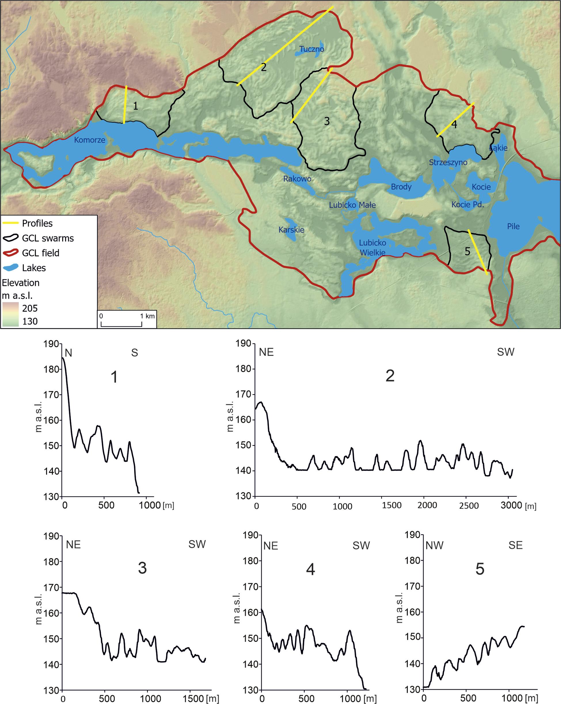
Similar trends were observed in Swarm 5, as illustrated in Figure 3A–C. At the lowest FT (FT = 1), intermediate landform types such as spur (14%), hollow (11%) and shoulder (3%) were predominant. As the FT value increased, the proportion of these classes systematically declined, with spur decreasing to 6% and hollow to 5% at FT = 3. Shoulder was the only category from this group that increased in area share (to 16%), likely due to the merging of adjacent pixels. Simultaneously, a marked rise was observed in the extent of flat forms (from 0% to 14%) and footslope (from 2% to 13%), which appear to subsume areas formerly classified under more localised categories. The proportion of ridge and valley forms also declined (ridge: 15% to 9%; valley: 12% to 8%). At FT = 3, more extensive and spatially coherent ridge–valley structures emerge, although at the expense of finer morphological detail. These shifts clearly illustrate the role of the FT parameter in controlling the level of generalisation: lower thresholds capture greater surface complexity, while higher thresholds facilitate the isolation of the principal axes of GCL ridges.
Landform classification in glacial curvilineations (GCL) swarm 5 using geomorphons and Topographic Position Index (TPI). A–C – geomorphons (FT = 1, 2, 3); D–F – TPI (neighbourhood size = 50, 75, 100 m). (FT – flatness threshold).
The classification trends observed across all swarms consistently demonstrate the role of the FT in terrain generalisation, with slope remaining the dominant category and ridge–valley contrasts becoming increasingly coherent at higher thresholds.
The TPI-based classification similarly reveals the scale sensitivity of landform detection. Results reveal systematic shifts in form composition when using three neighbourhood sizes (50, 75 and 100 cells). At smaller neighbourhoods (N = 50), slope dominates all swarms (up to 57%), but this share declines with increasing window size (N = 100: 34%). Conversely, ridge and valley forms become more prevalent at larger neighbourhood sizes. Valley coverage increases from 22% (N = 50) to 35% (N = 100) and ridge from 21% to 31%.
Swarm 5 exemplifies this trend: slope coverage decreases from 61% (N = 50) to 42% (N = 100), while valley and ridge increase from 19% and 20% to 27% and 31%, respectively (Fig. 3). This pattern suggests that smaller windows emphasise local relief – highlighting slopes – while larger windows smooth topography and enhance the detection of broader-scale ridge and valley systems. These findings underscore the significance of neighbourhood size selection in TPI analyses, particularly when identifying narrow, elongated glacial landforms such as GCLs.
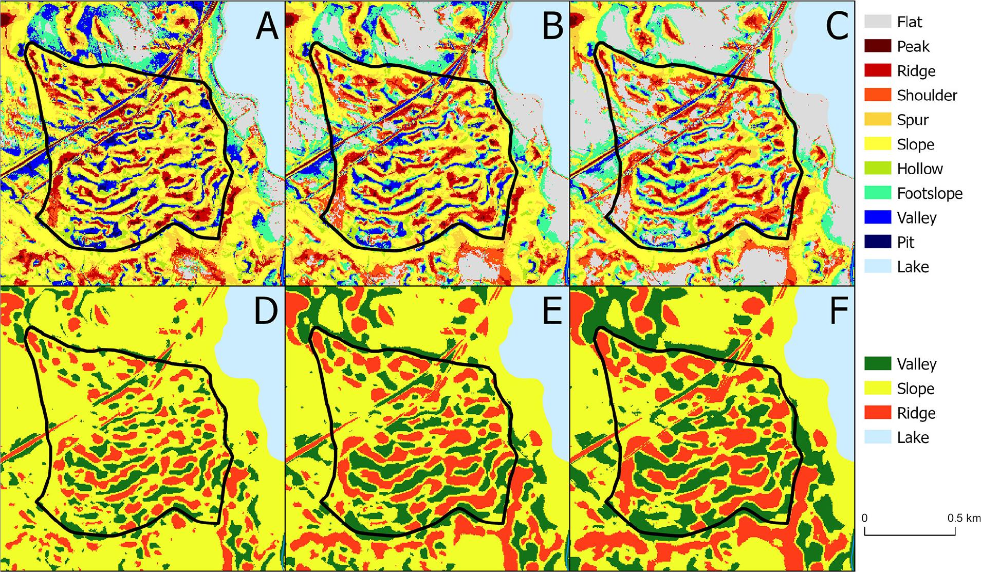
In terms of total area and form count, manual methods identify fewer features per swarm but with more extensive spatial coverage (Table 1). For example, Swarm 5 includes 15 manually defined GCLs covering 24.9% of the swarm area. Geomorphon methods detect more numerous features and greater total area coverage (up to 30.3%), though with increased fragmentation. TPI methods reveal high variability – Swarm 5 contains 43 forms at N = 50 (14.5% area) versus 25 forms at N = 100 (27.3% area), suggesting improved performance at larger window sizes (Fig. 4).
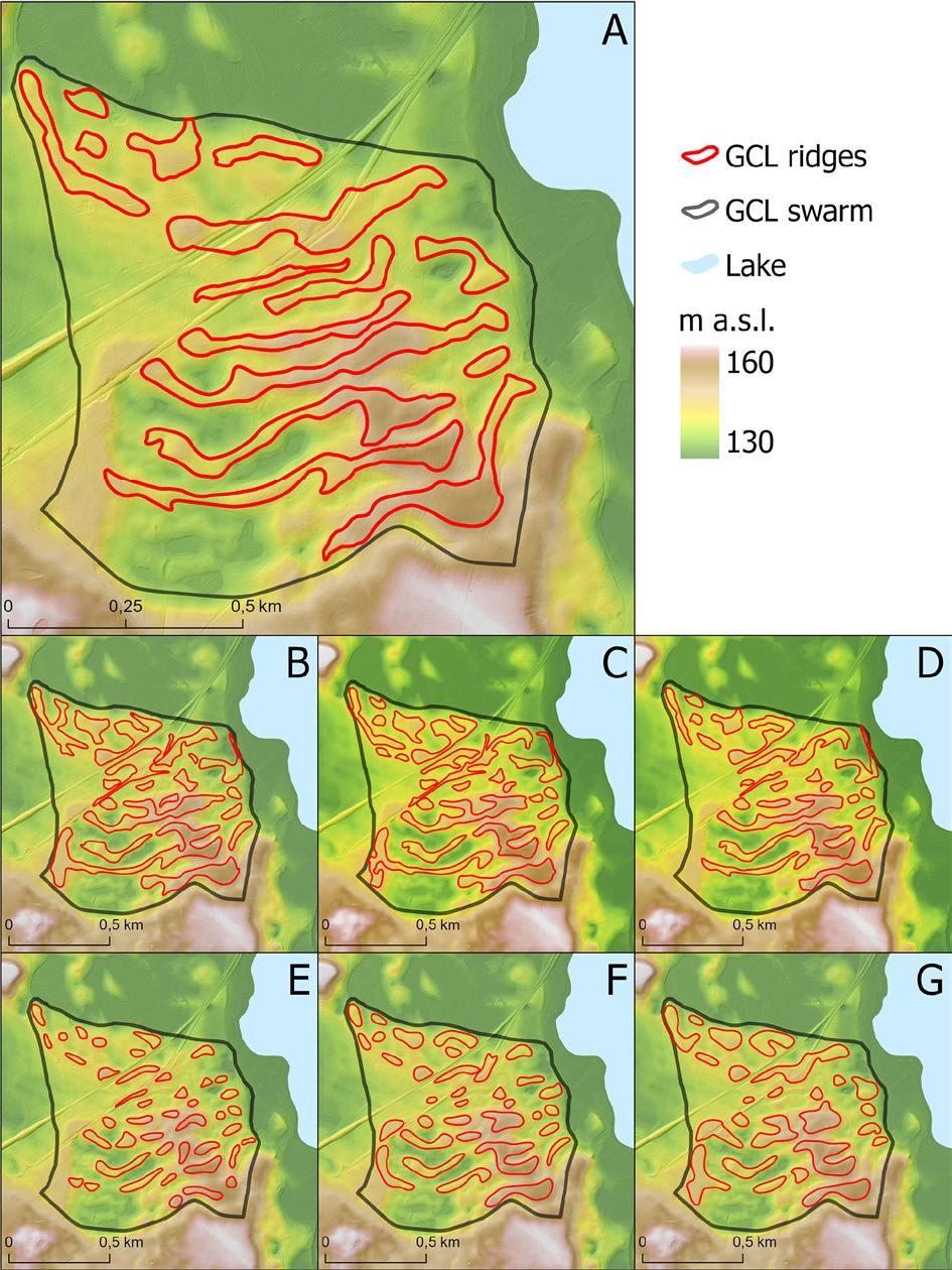
Comparison of GCL ridges outlines for GCL Swarm 5 derived using seven methods. A – manual delineation; B–D – geomorphons (FT = 1, 2, 3); E–G – TPI (neighbourhood size = 50, 75, 100 m). FT – flatness threshold; GCL – glacial curvilineation; TPI – Topographic Position Index.
Geomorphon-derived forms (FT = 1, 2, 3) demonstrate greater surface coverage and higher object counts. Swarm 5 illustrates this very well: the number of forms increases from 20 to 24 as FT rises, with surface area reaching 30.3% at FT = 1 (Table 2). This suggests that geomorphons are highly sensitive to minor topographic variations, but also prone to over-segmentation, potentially dividing a single manual form into multiple smaller ones. Nevertheless, in Swarm 5, geomorphons successfully capture the underlying structure of GCLs, and with an appropriately tuned FT (e.g. FT = 2), they can approximate the spatial distribution observed in manual mapping.
Morphometric parameters of glacial curvilineations (GCL) forms. (FT – flatness threshold).
| Swarm | Parameter | Unit | Manual | Geomorphons | Topographic Position Index | ||||||||||||||||||
|---|---|---|---|---|---|---|---|---|---|---|---|---|---|---|---|---|---|---|---|---|---|---|---|
| FT = 1 | FT = 2 | FT = 3 | N = 50 | N = 75 | N = 100 | ||||||||||||||||||
| Mean | Max | Min | Mean | Max | Min | Mean | Max | Min | Mean | Max | Min | Mean | Max | Min | Mean | Max | Min | Mean | Max | Min | |||
| 1 | Area | [ha] | 1.754 | 3.085 | 0.579 | 1.119 | 4.547 | 0.101 | 1.177 | 4.385 | 0.102 | 1.229 | 3.759 | 0.101 | 0.612 | 2.520 | 0.101 | 1.037 | 4.302 | 0.115 | 2.050 | 8.484 | 0.106 |
| Length | [m] | 428 | 819 | 212 | 243 | 875 | 25 | 263 | 886 | 21 | 284 | 698 | 21 | 150 | 566 | 14 | 197 | 669 | 30 | 311 | 1082 | 40 | |
| Hmean | [m a.s.l.] | 148 | 156 | 140 | 148 | 157 | 138 | 147 | 156 | 138 | 147 | 156 | 140 | 148 | 159 | 137 | 148 | 159 | 137 | 148 | 157 | 138 | |
| Hmax | 152 | 162 | 142 | 150 | 162 | 139 | 150 | 162 | 139 | 151 | 162 | 141 | 150 | 162 | 138 | 151 | 162 | 138 | 152 | 162 | 139 | ||
| Hmin | 141 | 149 | 134 | 143 | 154 | 133 | 143 | 152 | 133 | 143 | 152 | 134 | 144 | 154 | 136 | 144 | 154 | 136 | 143 | 153 | 134 | ||
| 2 | Area | [ha] | 1.072 | 6.374 | 0.104 | 1.041 | 5.920 | 0.107 | 0.966 | 5.114 | 0.101 | 0.809 | 4.910 | 0.101 | 0.474 | 2.503 | 0.101 | 0.709 | 8.611 | 0.100 | 1.090 | 9.429 | 0.103 |
| Length | [m] | 258 | 1151 | 44 | 225 | 901 | 25 | 216 | 898 | 14 | 191 | 903 | 14 | 124 | 533 | 21 | 148 | 1447 | 21 | 188 | 1422 | 21 | |
| Hmean | [m a.s.l.] | 148 | 157 | 140 | 147 | 156 | 140 | 147 | 156 | 140 | 147 | 157 | 140 | 148 | 158 | 141 | 148 | 156 | 141 | 148 | 156 | 141 | |
| Hmax | 151 | 161 | 141 | 150 | 161 | 141 | 150 | 161 | 141 | 150 | 161 | 141 | 150 | 161 | 142 | 150 | 161 | 142 | 151 | 161 | 142 | ||
| Hmin | 144 | 152 | 137 | 143 | 152 | 136 | 144 | 152 | 137 | 144 | 154 | 137 | 146 | 152 | 139 | 145 | 152 | 139 | 145 | 152 | 138 | ||
| 3 | Area | [ha] | 1.531 | 7.189 | 0.102 | 1.610 | 8.073 | 0.129 | 1.627 | 7.843 | 0.107 | 1.006 | 7.692 | 0.102 | 0.572 | 2.565 | 0.102 | 1.079 | 9.315 | 0.110 | 1.602 | 10.174 | 0.110 |
| Length | [m] | 298 | 1281 | 38 | 286 | 1142 | 28 | 298 | 1204 | 21 | 196 | 1034 | 14 | 137 | 513 | 28 | 191 | 1179 | 25 | 246 | 1170 | 28 | |
| Hmean | [m a.s.l.] | 148 | 155 | 142 | 148 | 155 | 140 | 148 | 154 | 140 | 147 | 156 | 140 | 148 | 156 | 139 | 147 | 154 | 140 | 147 | 153 | 140 | |
| Hmax | 151 | 164 | 144 | 151 | 164 | 141 | 151 | 164 | 141 | 150 | 164 | 141 | 150 | 164 | 140 | 150 | 164 | 141 | 150 | 164 | 141 | ||
| Hmin | 144 | 149 | 137 | 143 | 149 | 135 | 143 | 149 | 135 | 144 | 150 | 137 | 145 | 153 | 137 | 144 | 150 | 138 | 144 | 149 | 137 | ||
| 4 | Area | [ha] | 1.600 | 6.030 | 0.106 | 1.317 | 9.452 | 0.100 | 1.210 | 9.800 | 0.105 | 0.960 | 3.864 | 0.106 | 0.309 | 1.336 | 0.105 | 0.734 | 2.475 | 0.146 | 1.177 | 7.434 | 0.112 |
| Length | [m] | 382 | 985 | 62 | 263 | 1620 | 42 | 244 | 1594 | 57 | 205 | 547 | 55 | 95 | 292 | 35 | 157 | 506 | 42 | 208 | 905 | 55 | |
| Hmean | [m a.s.l.] | 146 | 151 | 141 | 146 | 150 | 142 | 145 | 150 | 141 | 146 | 152 | 141 | 146 | 154 | 139 | 146 | 154 | 138 | 146 | 152 | 141 | |
| Hmax | 149 | 157 | 145 | 148 | 157 | 143 | 147 | 157 | 143 | 147 | 157 | 142 | 147 | 157 | 139 | 148 | 157 | 142 | 148 | 157 | 142 | ||
| Hmin | 142 | 147 | 134 | 143 | 146 | 135 | 143 | 147 | 134 | 143 | 147 | 134 | 144 | 151 | 137 | 143 | 150 | 135 | 143 | 148 | 135 | ||
| 5 | Area | [ha] | 1.556 | 3.645 | 0.210 | 1.417 | 6.132 | 0.103 | 1.110 | 3.552 | 0.149 | 0.893 | 3.864 | 0.129 | 0.316 | 0.976 | 0.124 | 0.628 | 2.512 | 0.110 | 1.021 | 2.773 | 0.108 |
| Length | [m] | 411 | 839 | 57 | 300 | 1071 | 60 | 270 | 778 | 53 | 244 | 850 | 53 | 102 | 301 | 14 | 149 | 425 | 41 | 182 | 532 | 21 | |
| Hmean | [m a.s.l.] | 141 | 146 | 136 | 140 | 146 | 136 | 140 | 147 | 136 | 141 | 148 | 136 | 142 | 149 | 136 | 141 | 148 | 136 | 141 | 148 | 136 | |
| Hmax | 144 | 151 | 137 | 143 | 151 | 139 | 143 | 151 | 137 | 143 | 151 | 137 | 143 | 151 | 136 | 143 | 151 | 137 | 143 | 151 | 137 | ||
| Hmin | 136 | 138 | 134 | 137 | 142 | 132 | 137 | 140 | 132 | 137 | 141 | 132 | 139 | 146 | 135 | 138 | 143 | 134 | 138 | 142 | 134 | ||
TPI-based forms, in contrast, exhibit even greater variability in both number and area coverage. In Swarm 5, the highest count occurs at the smallest neighbourhood (N = 50) – 43 forms – but these cover only 14.5% of the area. At N = 100, the form counts drops to 25, while area coverage increases to 27.3%, nearly matching the manual delineation (Fig. 4, Table 2) indicating that TPI may approximate expert interpretation with appropriately selected parameters, though smaller neighbourhoods tend to cause excessive fragmentation, as shown in map D – forms appear shorter, more numerous and less spatially coherent.
Manually delineated GCLs served as a reference for evaluating form geometry across methods. These hand-mapped features are characterised by moderate surface area (1.07–1.75 ha on average), varied lengths (258–428 m) and narrow elevation ranges (Table 2). In Swarm 5, the average form area is 1.56 ha, length 411 m and elevations range from 136 m a.s.l. to 144 m a.s.l. These forms exhibit clear spatial structure and minimal fragmentation.
Geomorphon-derived forms, especially at FT = 3, show reduced area and length relative to manual forms, with increased segmentation. In Swarm 5, at FT = 1, forms average 1.42 ha and 300 m in length, decreasing to 1.11 ha and 270 m at FT = 3. Despite similar Hmean values (~140 m), these forms are more fragmented and sensitive to input parameters.
TPI-based forms show the highest level of fragmentation, particularly with smaller neighbourhoods. In Swarm 5, TPI (N = 50) yields a mean form area of only 0.32 ha and a mean length of 102 m – substantially smaller than manually obtained results. At N = 100, average area rises to 1.02 ha and length to 182 m, partially aligning with manual values, even though continuity and spatial coherence remain lower.
Across all swarms, manual delineations consistently yield higher median values for area and length, with low variance, reflecting expert selectivity and form cohesion. Automated methods, on the other hand, produce smaller, more fragmented forms, with greater variability, highlighting sensitivity to terrain heterogeneity. Hmean remains generally consistent (140–150 m), though automated methods sometimes trend slightly lower, particularly in Swarm 5, indicating a mild bias towards more recessed terrain (Fig. 5).
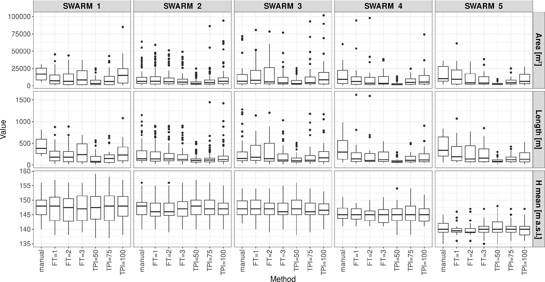
Distribution of selected morphometric characteristics of GCLs derived using different methods: geomorphons (FT = 1, 2, 3); TPI (neighbourhood size = 50, 75, 100 m). FT – flatness threshold; GCLs – glacial curvilineations; TPI – Topographic Position Index.
These results underscore the influence of method selection and parameterisation on the delineation and interpretation of GCLs. While automated approaches are better for scaling up geomorphometric analysis, their outputs differ markedly in form coherence, geometry and landscape sensitivity. The following section contextualises these findings by evaluating method strengths and limitations in light of glacial geomorphological interpretation.
This study does not aim to introduce novel landform classification techniques but rather to apply established geomorphometric tools – specifically geomorphons and the TPI – to a previously underexplored glacial landform type, GCLs. While the primary objective was to interpret the geomorphology of these features, the evaluation of automated delineation results also provides valuable insight into the broader applicability of such methods in complex postglacial landscapes.
Previous comparisons of geomorphon and TPI methods in various morphogenetic zones have highlighted differences in the performance of both techniques (Evans et al. 2016, Kramm et al. 2017, Jancewicz et al. 2022, Gawrysiak, Kociuba 2023, Gupta, Dixit 2024). Gawrysiak (2018) analysed terrain characteristics across several landscape types in Poland, including the young glacial zone, and compared classification results with geomorphological maps. His results, based on the Chełmno-Dobrzyń Lakeland and Toruń Basin, indicated moderate to high consistency between TPI and geomorphons in identifying convex forms. However, TPI often exaggerated the spatial extent of these forms, assigning them larger areas than geomorphons or morphological-hypsometric analyses would suggest. While both methods proved effective in distinguishing major morphogenetic units, their outputs diverged in detail, particularly for subtle glacifluvial features and eroded plateau margins.
In contrast, the GCLs in the Komorze Lake tunnel valley, which represent small-scale, regularly arranged ridge-trough systems typical of young glacial terrain, did not show significant area overestimation by TPI relative to geomorphons. This suggests that, for such finely structured landforms, careful parameterisation may outweigh the influence of the classification algorithm itself.
The comparison between geomorphon- and TPI-based automated delineation methods revealed some discernible tendencies in how each approach represents GCLs, both in terms of morphometric outputs and fidelity to manually refined interpretations. As illustrated in Figure 6, geomorphon-based delineations – particularly with a FT of 3 (FT = 3) – consistently showed the closest alignment with manual GCL mapping. FT = 3 showed no significant differences in percentage area and form count, and relatively low percent deviations in form area (+17.3%), percentage area (+6.4%) and form count (+87.8%). These results suggest that the FT = 3 method provides a more balanced representation of both spatial extent and feature density, indicating a relative advantage in preserving the integral shape and spatial coherence of GCL swarms.
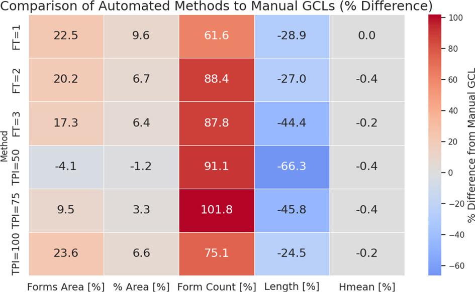
Percent differences between automated and manual glacial curvilineations (GCL) delineations across five GCL swarms. Geomorphon (flatness threshold FT = 1, 2, 3); Topographic Position Index (TPI) (neighbourhood size = 50, 75, 100 m) methods are compared. Warm colours indicate overestimation; cool colours indicate underestimation.
TPI-based methods, while effective at detecting ridge-like forms, demonstrated greater deviations from manual interpretations. Notably, TPI = 50 and TPI = 75 were prone to over-segmentation (Fig. 6), reflected in inflated form counts (+91.1% and +101.8%) and substantially reduced mean form lengths (–66.3% and –45.8%), indicating fragmented ridge continuity. TPI = 100, by contrast, revealed more moderate deviations and yielded form areas most similar to the manual benchmark, although there were notable differences across other metrics. These outcomes underscore the trade-offs associated with neighbourhood size: smaller analysis windows increase sensitivity to local variation but may distort the spatial integrity of elongated features, while larger windows enhance coherence at the cost of reduced specificity.
Manual delineation of GCLs in the Komorze valley underscores the interpretive advantages of expert-based mapping. The manually classified forms displayed coherent geometry, consistent morphometric properties and low spatial fragmentation. These outcomes affirm the continued relevance of manual mapping, particularly for subtle glacial landforms that require contextual awareness of form organisation and topographic continuity. However, automated approaches remain sensitive to terrain heterogeneity, particularly in young glacial landscapes like the Drawsko Lakeland, where glacial, fluvioglacial and postglacial processes converge (Dyba, Jasiewicz 2022). TPI methods, in particular, tended to over-segment morphologically subtle GCLs, highlighting limitations in elevation-only classification in topographically nuanced settings. These results support the notion that hybrid approaches – integrating automated classification with expert-guided interpretation – may offer the most robust framework for accurate landform mapping.
Although this study was not designed as a methodological benchmark, the results highlight the potential of automated techniques in broader geomorphological workflows. Geomorphons, in particular, offer promise as scalable screening tools – especially when paired with expert insight and parameter tuning. TPI remains valuable in larger-scale pattern recognition, but its limitations at finer scales necessitate careful calibration.
Future research should prioritise the testing of automated GCL delineation across a wider range of glaciated terrains, including those with different degrees of glacial modification. Integration with sedimentological and geophysical data may enhance interpretation accuracy, thus enabling a more comprehensive understanding of subglacial processes and landform genesis. The present study lays a foundation for such interdisciplinary approaches, emphasising the continued need to blend quantitative analysis with geomorphological reasoning.
This study evaluated the effectiveness of two automated geomorphometric methods – geomorphons and the TPI – in delineating GCLs within the Komorze tunnel valley in the Drawsko Lakeland, NW Poland. Using a manually refined dataset as a reference, the spatial characteristics of ridge forms produced by each method across five GCL swarms are compared.
The results highlight the interpretative reliability of the geomorphon approach, particularly with an FT of 3, in replicating the structure and distribution of GCLs. TPI-based methods were more sensitive to neighbourhood size and frequently over-fragmented the terrain, leading to inflated form counts and a reduction in spatial coherence. Though all methods produced comparable elevation ranges, only geomorphons nearly approximated the shape and extent of GCL ridges identified through manual interpretation.
Given the challenges of mapping low-relief landforms in young, morphologically diverse glacial landscapes, this study demonstrates that automated approaches, when carefully parameterised and validated, can effectively support geomorphological analysis. These findings reinforce the enduring value of expert-guided interpretation while showing that tools like geomorphons can meaningfully assist in identifying subtle features such as GCLs, especially at larger spatial scales. As geomorphometric frameworks evolve, a hybrid approach that balances automation with contextual insight will be crucial to advancing the study of glacial landscapes and their formative processes.