
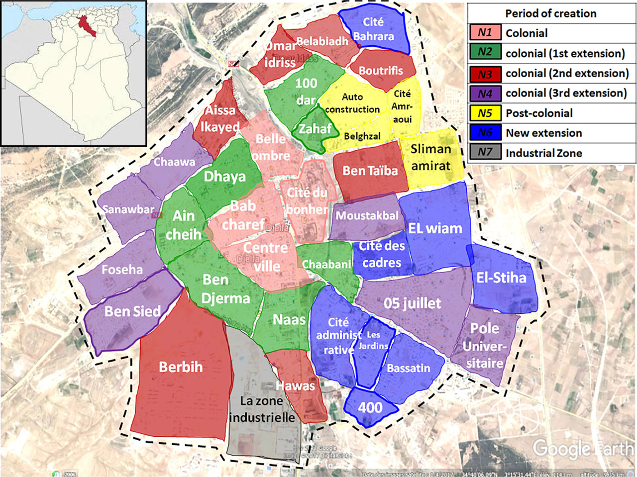
Fig. 1
Study area and the neighbourhoods of the city according to their period of creation.
Source: own composition based on Bouzidi et Boukhari 2013.
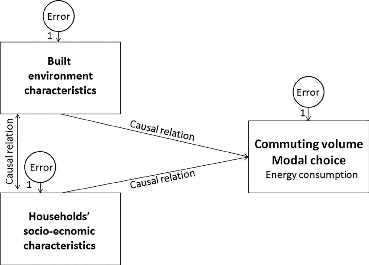
Fig. 2
Conceptual model explaining the need for commuting.
Table 1
Pearson's bivariate correlation.
| Commuting energy consumption (KWh × person−1 × year−1) | |||
|---|---|---|---|
| Correlation | Sig | No. | |
| Home-work distance (m) | 0.561* | 0.000 | 162 |
| Outward journey time (min) | 0.035* | 0.661 | 163 |
| Number of bus rotations | 0.247* | 0.004 | 136 |
| Built density | −0.135* | 0.133 | 125 |
| Plot ratio | −0.120* | 0.184 | 125 |
| Housing type (1: collective, 2: individual) | −0.153* | 0.051 | 164 |
| Distance from national road (m) | 0.256* | 0.003 | 136 |
| Distance to centre (m) | 0.280* | 0.001 | 133 |
| Block's area (m2) | 0.224* | 0.012 | 125 |
| Average number of floors | 0.143* | 0.112 | 125 |
| Mixed use index | −0.049* | 0.545 | 156 |
| Distance to public transport (housing zone) | −0.152* | 0.059 | 154 |
| Distance to public transport (work zone) | −0.145* | 0.064 | 164 |
| Round trip frequency | 0.118* | 0.141 | 156 |
| Profession (1: public, 2: liberal) | 0.169* | 0.031 | 163 |
| Respondent age | −0.265* | 0.005 | 109 |
| Respondent's education level | 0.107* | 0.183 | 156 |
| Household's education level | 0.102* | 0.541 | 138 |
| Income | 0.136* | 0.082 | 163 |
| Household's average age | −0.307* | 0.064 | 137 |
| Number of cars owned | 0.379* | 0.000 | 163 |
| Occupancy rate per housing | −0.073* | 0.418 | 126 |
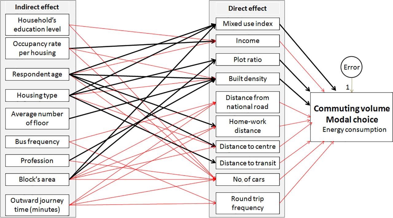
Fig. 3
The hypothesised model.
In red: positive causal relation; in black: negative causal relation
Source: own study.
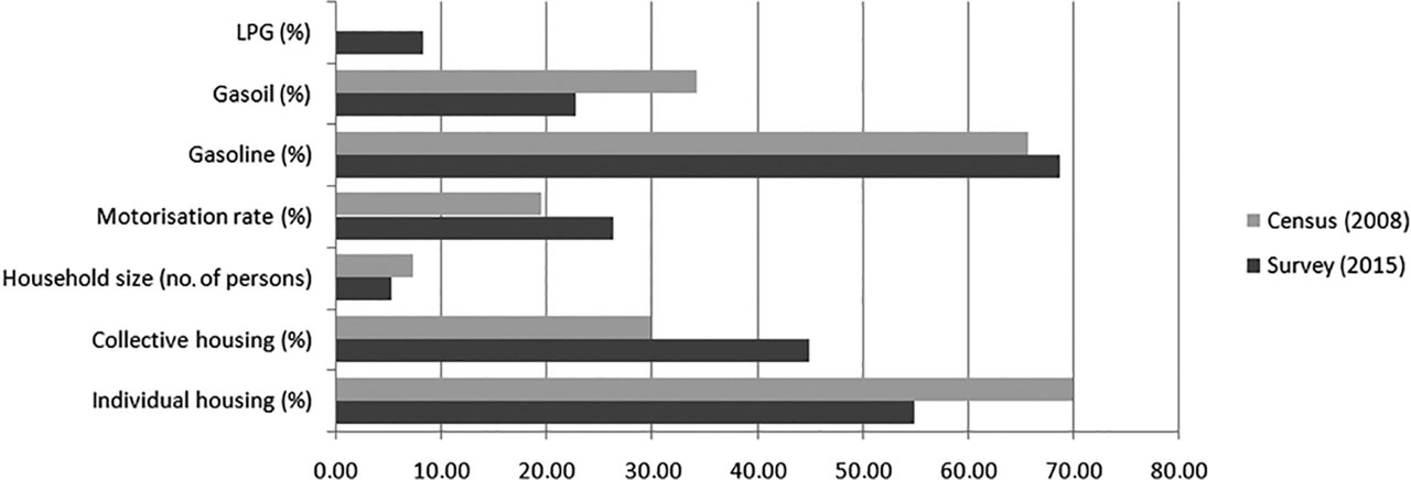
Fig. 4
Comparison between the survey and census data.
LPG – liquefied petroleum gas
Source: own study.
Table 2
Descriptive statistics.
| Variables | N | Variable type | Minimum | Maximum | Average | SD |
|---|---|---|---|---|---|---|
| Accessibility | ||||||
| Outward journey time (min) | 175 | Continuous | 2 | 200 | 20.59 | 18.26 |
| Home–work distance (m) | 162 | Continuous | 50 | 18,000 | 2,206.91 | 1,966.96 |
| Number of bus rotations | 150 | Continuous | 0 | 3 | 1.20 | 0.556 |
| Density | ||||||
| Plot ratio* | 139 | Continuous | 0.17 | 1.00 | 0.59 | 0.32 |
| Built density* | 139 | Continuous | 0.60 | 3.20 | 2.02 | 0.74 |
| Design | ||||||
| Distance to centre (m)* | 148 | Continuous | 17.59 | 2,659.18 | 1,219.54 | 696.57 |
| Distance from national road (m)* | 151 | Continuous | 25.62 | 2,569.23 | 1,163.83 | 629.94 |
| Average number of floors. (n)* | 139 | Continuous | 2.00 | 6.00 | 3.79 | 1.08 |
| Block's area (m2)* | 139 | Continuous | 770 | 36.061 | 7,398.83 | 9,150.32 |
| Housing type (1: collective, 2: individual) | 184 | Nominal | 1 | 2 | 1.54 | 0.50 |
| Distance to public transport | ||||||
| Distance to public transport (housing zone) (0: <300, 4: >1 km) | 173 | Ordinal | 1.00 | 4.00 | 2.3237 | 0.98 |
| Distance to public transport (work zone) (0: <300, 4: >1 km) | 172 | Ordinal | 0.00 | 4.00 | 1.6919 | 0.97 |
| Bus frequency | 184 | Continuous | 0.00 | 5.00 | 2.4620 | 1.56 |
| Diversity | ||||||
| Mixed use index (from 5 to 40)* | 175 | Continuous | 12 | 36 | 24.23 | 5.38 |
| Households’ SE characteristics | ||||||
| Household's average age* | 42 | Continuous | 16.33 | 43.80 | 27.1681 | 8.44 |
| Respondent age | 120 | Continuous | 27 | 70 | 43.95 | 10.82 |
| Round-trip frequency | 172 | Continuous | 1 | 4 | 1.66 | 0.51 |
| Household's education level | 46 | Continuous | 2.00 | 5.00 | 3.5230 | 0.77 |
| Respondent's education level | 174 | Ordinal | 0 | 4 | 3.26 | 1.06 |
| Number of cars owned | 184 | Continuous | 0 | 2 | 0.60 | 0.57 |
| Profession (1: public, 2: liberal) | 181 | Nominal | 1 | 3 | 1.19 | 0.52 |
| Income (from 15,000 to + 60,000 Da) | 181 | Ordinal | 1 | 4 | 2.15 | 0.95 |
| Occupancy rate per housing. | 139 | Continuous | 2 | 12 | 5.34 | 1.87 |
| Modal share | ||||||
| Public transport (TC (1: TC, 0: other) | 184 | Nominal | 0.00 | 1.00 | 0.31 | 0.46 |
| Car (1: Voiture, 0: other) | 184 | Nominal | 0.00 | 1.00 | 0.26 | 0.44 |
| Walking (1: MAP, 0: other) | 184 | Nominal | 0.00 | 1.00 | 0.42 | 0.49 |
[i] SD – standard deviation, SE – socio-economic
[ii] Source: Boukarta and Berezowska-Azzag (2020).
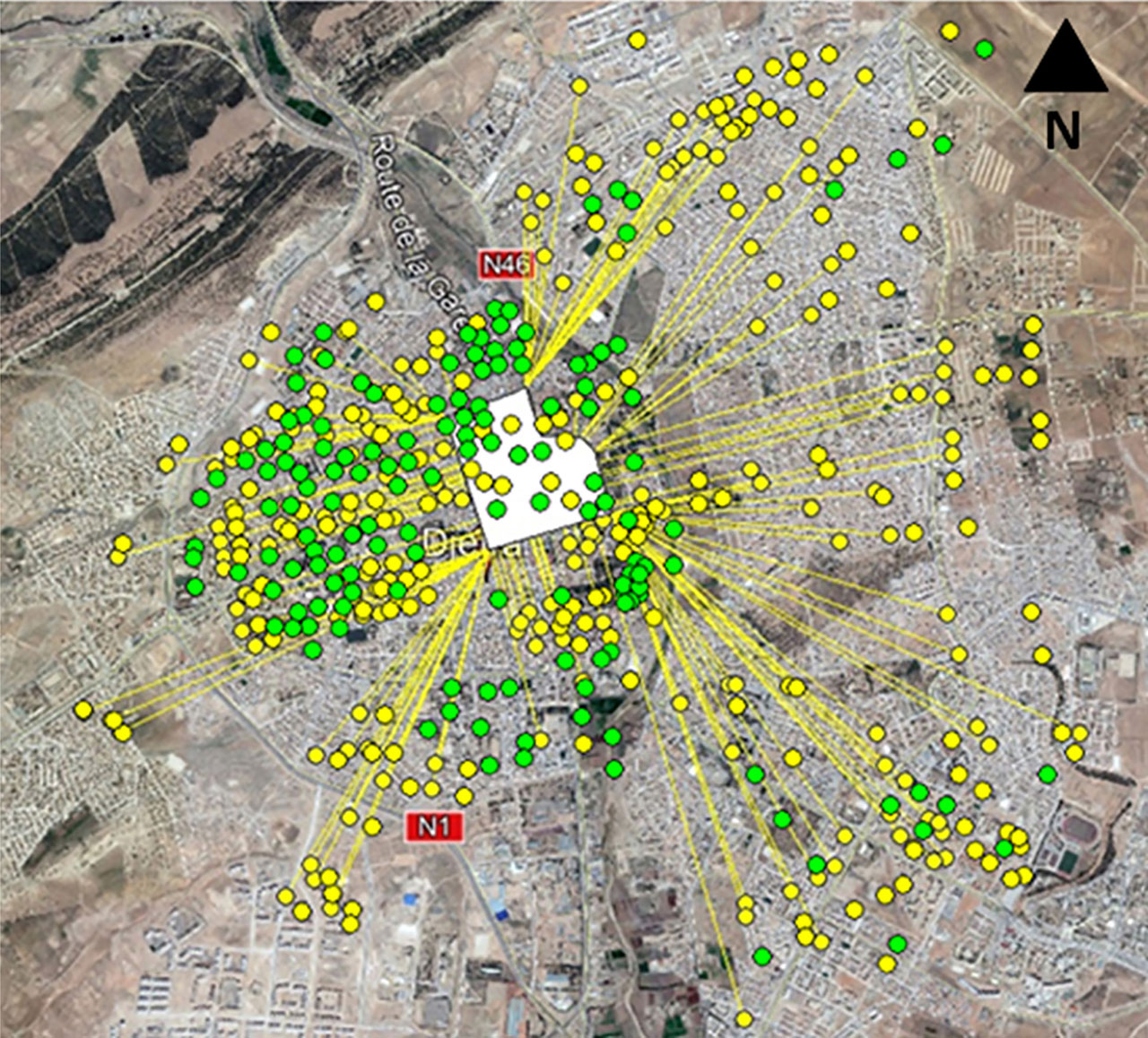
Fig. 5
Employment and housing locations.
green: workplace, yellow: housing, white: centre of the city
Source: authors’ compilation based on Google Earth (2015).
Table 3
Fuel conversion to kWh per km per person.
| Means of commuting | ||||
|---|---|---|---|---|
| Car | Bus | |||
| Fuel type | Diesel | Petrol | LPG | Diesel |
| Consumption (L × km−1) | 0.063* | 0.075* | 0.075* | 0.2** |
| Rate of occupation per vehicle | 1.27* | 1.27* | 1.27* | 28** |
| Density (Tonne/m3) | 0.825**** | 0.735***** | 0.55 | 0.825 |
| Conversion factor 1 (T fuel – >Toe)*** | 1,015 | 1,054 | 1,084 | 1,015 |
| Conversion factor 2 (Toe – >KWh) | 11,630*** | |||
| Consumption KWh × km−1 | 0.61 | 0.68 | 0.52 | 1.95 |
| Consumption KWh per person per Km per one-way trip | 0.48 | 0.53 | 0.41 | 0.07 |
| Consumption KWh per person per Km per year (225 day) | 108 | 119.25 | 92.25 | 15.75 |
Table 4
Descriptive statistics of the energy consumption generated by commuting to work.
| Minimum | Maximum | Average | SD | |
|---|---|---|---|---|
| Home-to-work distance | 50 | 18,000 | 2,206.91 | 1,966.96 |
| Daily consumption (kWh × person−1) | 0.00 | 3.60 | 0.4853 | 0.788 |
| Annual consumption (kWh × person−1 × an) | 0.00 | 810.00 | 109.1854 | 177.31 |
[i] SD – standard deviation.
[ii] Source: own study.
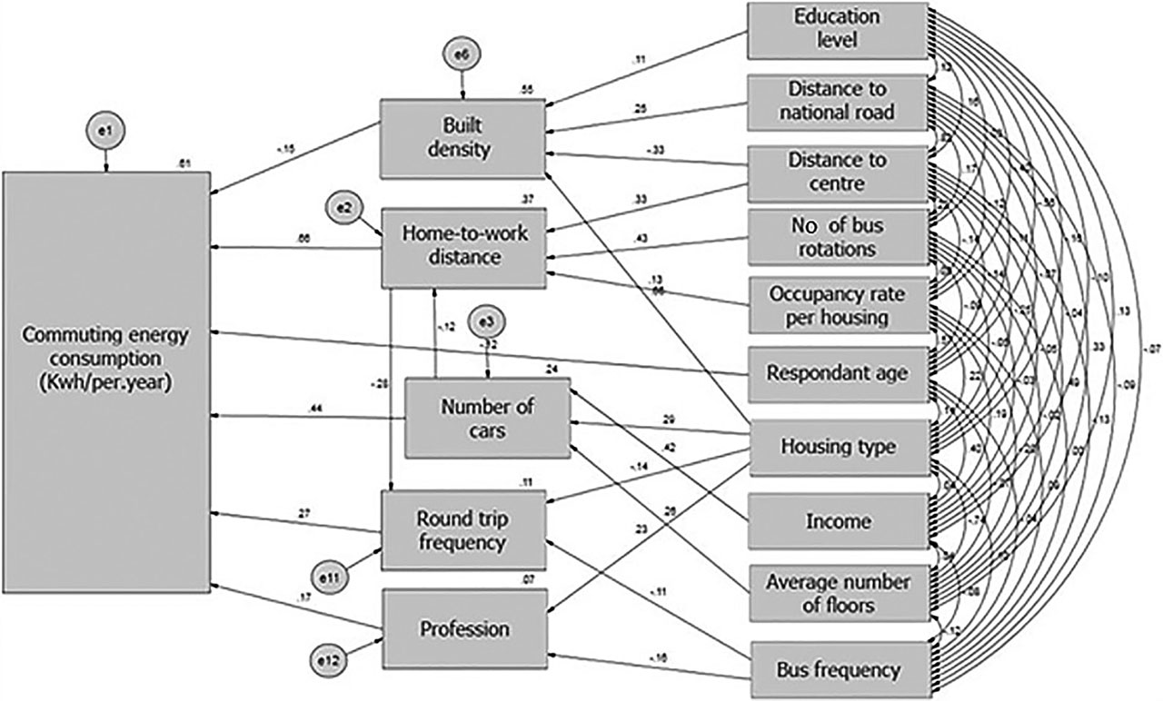
Fig. 6
Direct effects of driving factors explaining the energy consumption generated by commuting. R2 = 0.61.
Source: own compilation.
Table 5
Fit indices of the energy consumption of commuting model.
| df | c2 | Probability level | RMSEA | NFI | CFI | |
|---|---|---|---|---|---|---|
| Commuting energy consumption model | 53 | 47.785 | 0.677 | 0.000 | 0.948 | 1.000 |
[i] CFI – Comparative Fit Index, NFI – Normal Fit Index, RMSE – Root Mean Square Error
[ii] Source: own study.
Table 6
Direct effects between driving factors.
| Effect | P | |||
|---|---|---|---|---|
| Number of cars | < – - | Income | 0.425 | *** |
| Number of cars | < – - | Number of floors | 0.255 | 0.019** |
| Number of cars | < – - | Housing type | 0.295 | 0.004** |
| Home-to-work distance | < – - | Distance to centre | 0.330 | *** |
| Home-to-work distance | < – - | Number of bus rotation | 0.427 | *** |
| Home-to-work distance | < – - | Occupancy rate per housing | 0.130 | 0.070* |
| Home-to-work distance | < – - | Number of cars | −0.117 | 0.071* |
| Built density | < – - | Distance to national road | 0.252 | 0.014** |
| Profession | < – - | Bus frequency | −0.155 | 0.032** |
| Built density | < – - | Distance to centre | −0.331 | 0.002** |
| Built density | < – - | Education level | 0.111 | 0.061* |
| Profession | < – - | Housing type | 0.227 | 0.002** |
| Round trip frequency | < – - | Housing type | −0.139 | 0.057* |
| Built density | < – - | Housing type | 0.664 | *** |
| Round trip frequency | < – - | Bus frequency | −0.105 | 0.149 |
| Round trip frequency | < – - | Home-to-work distance | −0.285 | *** |
| Energy consumption (kWh × person−1 × year−1) | < – - | Home-to-work distance | 0.661 | *** |
| Energy consumption (kWh × person−1 × year−1) | < – - | Profession | 0.165 | *** |
| Energy consumption (kWh × person−1 × year−1) | < – - | Round trip frequency | 0.271 | *** |
| Energy consumption (kWh × person−1 × year−1) | < – - | Number of cars | 0.448 | *** |
| Energy consumption (kWh × person−1 × year−1) | < – - | Built density | −0.145 | 0.007** |
| Energy consumption (kWh × person−1 × year−1) | < – - | Respondent age | −0.119 | 0.032** |
Table 7
Direct and indirect effects of the driving factors of energy consumption generated by commuting.
| Effect | Number of cars | Home-to-work distance | Round trip frequency | Profession | Built density | Energy consumption (kWh person−1 × year−1) | |
|---|---|---|---|---|---|---|---|
| Number of floors | Direct | 0.255 | 0.000 | 0.000 | 0.000 | 0.000 | 0.000 |
| Indirect | 0.000 | −0.030 | 0.009 | 0.000 | 0.000 | 0.097 | |
| Total | 0.255 | −0.030 | 0.009 | 0.000 | 0.000 | 0.097 | |
| Housing type | Direct | 0.295 | 0.000 | −0.139 | 0.227 | 0.664 | 0.000 |
| Indirect | 0.000 | −0.035 | 0.010 | 0.000 | 0.000 | 0.016 | |
| Total | 0.295 | −0.035 | −0.129 | 0.227 | 0.664 | 0.016 | |
| Income | Direct | 0.425 | 0.000 | 0.000 | 0.000 | 0.000 | 0.000 |
| Indirect | 0.000 | −0.050 | 0.014 | 0.000 | 0.000 | 0.161 | |
| Total | 0.425 | −0.050 | 0.014 | 0.000 | 0.000 | 0.161 | |
| Occupancy rate per housing | Direct | 0.000 | 0.130 | 0.000 | 0.000 | 0.000 | 0.000 |
| Indirect | 0.000 | 0.000 | −0.037 | 0.000 | 0.000 | 0.076 | |
| Total | 0.000 | 0.130 | −0.037 | 0.000 | 0.000 | 0.076 | |
| Bus rotation | Direct | 0.000 | 0.427 | 0.000 | 0.000 | 0.000 | 0.000 |
| Indirect | 0.000 | 0.000 | −0.122 | 0.000 | 0.000 | 0.249 | |
| Total | 0.000 | 0.427 | −0.122 | 0.000 | 0.000 | 0.249 | |
| Distance to centre | Direct | 0.000 | 0.330 | 0.000 | 0.000 | −0.331 | 0.000 |
| Indirect | 0.000 | 0.000 | −0.094 | 0.000 | 0.000 | 0.241 | |
| Total | 0.000 | 0.330 | −0.094 | 0.000 | −0.331 | 0.241 | |
| Number of cars | Direct | 0.000 | −0.117 | 0.000 | 0.000 | 0.000 | 0.448 |
| Indirect | 0.000 | 0.000 | 0.033 | 0.000 | 0.000 | −0.068 | |
| Total | 0.000 | −0.117 | 0.033 | 0.000 | 0.000 | 0.379 | |
| Education level | Direct | 0.000 | 0.000 | 0.000 | 0.000 | 0.111 | 0.000 |
| Indirect | 0.000 | 0.000 | 0.000 | 0.000 | 0.000 | −0.016 | |
| Total | 0.000 | 0.000 | 0.000 | 0.000 | 0.111 | −0.016 | |
| Bus frequency | Direct | 0.000 | 0.000 | −0.105 | −0.155 | 0.000 | 0.000 |
| Indirect | 0.000 | 0.000 | 0.000 | 0.000 | 0.000 | −0.054 | |
| Total | 0.000 | 0.000 | −0.105 | −0.155 | 0.000 | −0.054 | |
| Distance to national road | Direct | 0.000 | 0.000 | 0.000 | 0.000 | 0.252 | 0.000 |
| Indirect | 0.000 | 0.000 | 0.000 | 0.000 | 0.000 | −0.037 | |
| Total | 0.000 | 0.000 | 0.000 | 0.000 | 0.252 | −0.037 | |
| Home-to-work distance | Direct | 0.000 | 0.000 | −0.285 | 0.000 | 0.000 | 0.661 |
| Indirect | 0.000 | 0.000 | 0.000 | 0.000 | 0.000 | −0.077 | |
| Total | 0.000 | 0.000 | −0.285 | 0.000 | 0.000 | 0.584 | |
| Respondent age | Direct | 0.000 | 0.000 | 0.000 | 0.000 | 0.000 | −0.119 |
| Indirect | 0.000 | 0.000 | 0.000 | 0.000 | 0.000 | 0.000 | |
| Total | 0.000 | 0.000 | 0.000 | 0.000 | 0.000 | −0.119 | |
| Round–trip frequency | Direct | 0.000 | 0.000 | 0.000 | 0.000 | 0.000 | 0.271 |
| Indirect | 0.000 | 0.000 | 0.000 | 0.000 | 0.000 | 0.000 | |
| Total | 0.000 | 0.000 | 0.000 | 0.000 | 0.000 | 0.271 | |
| Profession | Direct | 0.000 | 0.000 | 0.000 | 0.000 | 0.000 | 0.165 |
| Indirect | 0.000 | 0.000 | 0.000 | 0.000 | 0.000 | 0.000 | |
| Total | 0.000 | 0.000 | 0.000 | 0.000 | 0.000 | 0.165 | |
| Built density | Direct | 0.000 | 0.000 | 0.000 | 0.000 | 0.000 | −0.145 |
| Indirect | 0.000 | 0.000 | 0.000 | 0.000 | 0.000 | 0.000 | |
| Total | 0.000 | 0.000 | 0.000 | 0.000 | 0.000 | −0.145 |
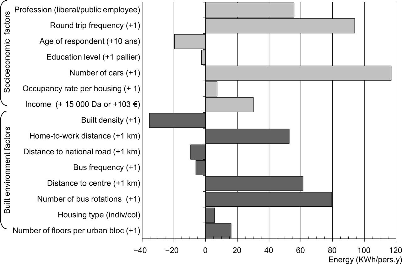
Fig. 7
Effect of SE and BE driving factors per unit of measurement on energy consumption of commuting to work.
BE – built environment, SE – socio-economic
Source: own compilation.
Table A1
Description of the papers chosen for the literature review.
| Authors | Country | Period | Data sources | Study scale | Sensitivity analysis method | Sample size | Mobility type | drivers | explanatory power of the modal | |||
|---|---|---|---|---|---|---|---|---|---|---|---|---|
| C | S | L | SE | BE | ||||||||
| Van Acker and Witlox (2010) | Belgium | 2000–2001 | Survey on behaviour of travellers in Ghent on people aged 18 and over. | City | SEM | 2,500 households | × | × | × | × | × | R2 = 20.1% |
| Breheny (1995) | UK – Wales | 1961–1991 | Aggregated data from Ecotec project (1993). | National | Interpolation from data from Ecotec project (1993). | Ecotec project sample (1993) | × | × | × | × | – | |
| Brownstone and Golob (2008) | California | 2001 | National Household Transportation Survey. Aggregate data. | National | SEM | 2,079 households | × | × | × | × | × | R2 = 0.37 and 0.42 |
| Calabrese et al. (2012) | Massachusetts, USA | 2011 | Deducted by detecting signal of mobile phones carried out by AirSag. | Metropolitan area | Multiple linear regression | 1,101 households | × | × | × | × | × | R2 = 49.40% and 56.48% |
| Newman et al. (1989) | 32 cities of different countries | 1980 | Collection of fuel consumption data and calculation of density excluding rural areas. Urban planning agency of different countries. Aggregate data. | City | Bivariate correlation analysis | 32 cities | × | × | × | × | × | / |
| Cervero and Murakami (2010) | USA | 2003 | Data collected from Highway Statistics. Department of Commerce. | National | SEM | 370 urban areas | × | × | × | × | CFI (>0: 900) 0.969 NFI (>0: 950) 0.961 NNFI (>0: 900) 0.942 | |
| Cervero and Radisch (1995) | USA | 1990–1991 | Bay Area Travel questionnaire survey. | Neighbourhood | Binary logistic regression | 2 Neighbourhoods: 620 households for non commuting. And 840 households for commuting | × | × | × | × | × | Pseudo R2 = 0.29, Predicted cases = 88.6%. |
| Chen et al. (2007) | NY, USA | 1997/1998 | Household survey | Metropolitan area | SEM | 2,089 trips | × | × | × | R2 = 0.45 and 0.58 | ||
| Dargay (2004) | UK | 1970–1995 | Surveys of family spending. | National | Semi-logistic regression | 256 pseudo panels | × | × | × | × | × | R2 = 0.989 |
| Dieleman et al. (2002) | Netherlands | 1996 | National Mobility Survey in the Netherlands | National | Multinomial logistic regression | 70,000 households | × | × | × | × | × | R2 = 0.31 |
| Ding et al. (2017) | Baltimore USA | 2001 | Household survey | Metropolitan area | SEM | 3,519 households | × | × | × | / | ||
| Feng et al. (2013) | China and Netherlands | 2008 | Household survey on mobility in both countries. | City | Multiple linear regression | 2,989 respondents for 10 districts in China and 1,322 respondents for Randstad. | × | × | × | × | × | China: R2 = 0.115 Randstad R2 = 0.124 |
| Handy et al. (2005) | California (US) | 2003 | E-mail questionnaire carried out on eight neighbourhoods. | District in metropolitan area | Linear regression | 1,466 respondents | × | × | R2 = 0.16 R2 adjusted = 154 | |||
| Holden and Norland (2005) | Oslo, Borway | 2003 | Questionnaire distributed by mail. | Regional | linear regression | 650 for daily trips, 778 for leisure travel, <100 respondents per zone (eight zones selected for the study). | × | × | × | × | R2 = 0.231 for commuting | |
| Karathodorou et al. (2010) | 42 countries | 1995 | Millennium Cities Database for Sustainable Transport (1999) for 100 countries. And car occupancy from Mobility in Cities database (2006). | Cities | Linear regression | 84 cities | × | × | × | × | R2 = 0.61 | |
| Khan et al. (2014) | Seatle, USA | 2006 | Questionnaires/Puget Sound Regional Council | Metropolitan area | Regression modelling | 10,510 respondents of 4,741 households. | × | × | × | × | / | |
| Kitamura et al. (1997) | San Francisco, USA | 1994 | Questionnaire, And land use information is obtained from the Metropolitan Transportation Commission. | Neighbourhood | Multiple linear regression | 5 Neighbourhoods, 640 respondents, | × | × | × | × | R2 = 0.2125 | |
| Limtanakool et al. (2006) | Netherlands | 1996 | National Mobility Survey conducted by telephone interview and questionnaire | Regional | Binary logistic regression | Commuting: 2,326 Shopping: 932 Leisure: 3,072 | × | × | × | × | × | |
| Ma et al. (2014) | China | 2007 | Questionnaires | Neighbourhoods | Logistic regression | 60 households, 699 trips of 10 neighbourhoods. | × | × | × | × | × | Pseudo R2 = 0.16 |
| Manaugh et al. (2009) | Montréal, Canada | 2003 | Origin-destination survey, | Neighbourhoods | Linear regression | 17,000 trips | × | × | × | SE: R2 = 0.06. SE+BE modal: R2 = 0.40 | ||
| Marique (2013) | Belgium | 2001 | 2001 SE survey | National | Multiple linear regression | 966.247 respondents. | × | × | × | R2 = 0.457 | ||
| Næss (2010) | Hangzhou, China | 2005 | Qualitative interview and questionnaire in 40 urban areas. | Urban zone | Multiple linear regression | 28 interviews 3,150 questionnaire respondents. | × | × | × | R2 = 0.189 | ||
| Naess (2014) | Hangzhou, China and Copenhague, Danemark | 2005 | Interview and questionnaire | Regional | Linear regression | 1932 et 3150 questionnaire | × | × | × | Copenhague R2 = 0.233 Hangzhou R2 = 0.095 | ||
| Pan et al. (2009) | Shanghai, China | 2001 | Questionnaires | Neighbourhood | Multiple logistic regression | 1,709 respondents in 4 Neighbourhoods | × | × | × | × | Pseudo R2 = 0.2714 | |
| Zhang et al. (2014) | Zhongshan, China | 2010 | Questionnaires | Neighbourhoods | Linear regression | 25,618 respondents | × | × | × | × | × | Pseudo R2 = 0.2823 |
| Bakour (2016) | Algiers, Algeria | 2004 | Household survey conducted by an organisation | City | Linear regression | 1,200 respondents | × | R2 = 0.5 à 0.9 | ||||
[i] BE – built environment, C – commuting, CFI – Comparative Fit Index, L – leisure, NFI – Normal Fit Index, S – shopping, SE – socio-economic, SEM – structural equation modelling
[ii] Source: own compilation.