

1. Introduction
The main challenge of rule-based systems is to consider the imprecision of the handled knowledge. It becomes a necessity since humans generally provide this type of data. It is no longer adequate to use Modus Ponens, which for a rule “If X is then Y is ”, it can only infer with an observation equal to the rule premise “X is ”. Therefore, approximate reasoning was proposed by Zadeh [1] in fuzzy context [2] in order to consider imprecise knowledge in the inference process. It is based on the generalization of Modus Ponens of classical logic, called Generalized Modus Ponens (GMP). The general schema of GMP is as follows:
where X and Y are linguistic variables and , , and are predicates.In classical logic, a rule is triggered only if there is a perfect match between its antecedent “X is ” and the observation. However, with GMP, an observation X is “ ” can differ from the antecedent “X is ”. And thus, the result “Y is ” will be not equal to the rule consequence “Y is ”.
The aim is to determine the conclusion “Y is ” so that it will be as close as possible to what an expert would decide. For that purpose, some authors [3] proposed criteria that should be verified by the conclusion to consider that it is valid and effective, and this was in the fuzzy context. In [4], the authors proposed the following generalization of approximate reasoning axiomatics which appeared in [3]:
This set of criteria describes the behavior that any approach of approximate reasoning should have, with the aim of obtaining relevant and coherent conclusions. Criterion I ensures the verification of classical Modus Ponens. Indeed, when the observation is equal to the rule premise , the conclusion must also be equal to the rule conclusion . This is a natural and logical behavior that is in concordance with classical logic as well as human thinking. Criterion II-1 and II-2 are interested in the case where the observation is a reinforcement of the premise. So, two positions can be adopted. The first one is to consider that the inference conclusion must also be a reinforcement of the rule conclusion . Whereas the second one imposes that the inference conclusion is equal to the rule conclusion . In effect, the choice between criterion II-1 and criterion II-2 depends on the causality between the premise and the conclusion of the rule. For example, with the rule “If a tomato is red then it is ripe”, we know that the more a tomato is red, the more it is ripe. With the observation “the tomato is very red” we can conclude that “The tomato is very ripe”. However, the expert can choose to have a cautious attitude by keeping as inference conclusion the rule conclusion as it is without considering the reinforcement of the observation. For example, with the rule “If the fog is slight then the speed is high” and the observation “The fog is very slight”, it is more adequate to deduce that “The speed is high” rather than “The speed is very high”. Indeed, following the reinforcement of the premise can, in this case, create a risk of accident. Finally, criterion III focuses on the case where the observation is a weakening of the premise. In that case, the inference conclusion must also be a weakening of the rule conclusion .
According to these criteria, two types of approximate reasoning can be released [3]:
These types are differentiated by the behavior of approximate reasoning when the observation is a reinforcement of the antecedent. The first adopts criterion II-1, and the second adopts criterion II-2. Criteria I and III must be checked in any case. The approximate reasoning type is fixed by the expert, who is knowledgeable of the nature of manipulated data and their behavior. Indeed, the type depends on the causality between the antecedent and the conclusion, which can only be evaluated by the expert.
Fuzzy reasoning has proven its performance in several applications, especially in fuzzy controls [5,6,7,8,9]. But some disadvantages of fuzzy set theory were pointed out by many researchers [10,11,12,13,14,15,16]. The principal limit is the numerical definition of fuzzy sets’ universe, which complicates the formalization of abstract terms like beautiful, intelligent, etc., since they do not have a numerical universe. Moreover, in fuzzy rule-based systems, it remains a problem to have a linguistic interpretation of the fuzzy set , the result of the inference. For that, multi-valued logic [13, 17,18,19,20] has been defined in order to handle imprecise knowledge in a symbolic way. This logic, as fuzzy logic, allows treating imprecise knowledge by authorizing intermediate degrees between the full membership and the non-membership. As proposed by De Glas [14], it is based on multi-sets theory. It evaluates knowledge imprecision in a qualitative way, which is more natural and is part of human thinking.
We focus in our work on approximate reasoning in the context of symbolic multi-valued logic. As a result of our bibliographic research within the framework of symbolic multi-valued logic, we have found that only the work [21] considers the axiomatics and the typology (3) to define approximate reasoning approaches. Indeed, two Generalized Modus Ponens for multi-valued knowledge have been proposed: the first one is of type 1, and the second is of type 2. The proposed approximate reasoning of type 1 was studied and extended in other works [22, 23]. It was also applied and used in a diagnosis aid system for autism [24,25,26] and has given very satisfactory results. The success of this system is due first to the verification of axiomatics. And also, psychiatry handles principally abstract data, where symptoms are non-measurable and are based mainly on the perception of doctors. Using symbolic multi-valued logic in that environment is then appropriate compared to fuzzy logic.
We are interested in this paper in another problem that concerns the form of manipulated predicates in symbolic approximate reasoning of type 2. In main and known approaches of symbolic approximate reasoning [10, 21, 27], all the multi-sets of the knowledge base must have the same degree scale. This may present a limit for the user in the sense that he will not be free in the definition of the multi-sets of the system. For that, our aim in this paper is to give a new model of approximate reasoning that can consider multi-sets that do not necessarily have the same scale base. We also treat another problem in the inference process, which is the form of rules. Indeed, experts can express rules that are not simple. For example, the antecedent of a rule can be complex, so that is composed of a conjunction or a disjunction of propositions. Another inference model is then proposed to deal with these types of rules.
This paper is organized as follows. In section 2., we present the symbolic multi-valued logic, which represents the context of our work. We also illustrate some reasoning models in that context and present the model of approximate reasoning of type 2. Section 3. gives proofs that this inference schema checks the axiomatics of approximate reasoning. We then propose in Section 4. an improvement of our multi-valued approximate reasoning for multi-bases knowledge. In section 5., we treat the case of reasoning with complex rules. We extend this reasoning so that it supports the simultaneous presence of complex rules and multi-base knowledge in Section 6.. A discussion is given in Section 7., we finally complete this paper with a conclusion in Section 8..
2. Reasoning in symbolic context
We present in this section the symbolic multi-valued logic according to the definition of Akdag et al. [17]. Then, we present some approximate reasoning models in that context.
2.1. Symbolic multi-valued logic
Symbolic multi-valued logic was proposed as a solution to consider imprecise knowledge in intelligent systems. Unlike classical logic, it allows assigning to an affirmation a value that is between the True and the False. Thus, the set of degrees forms an ordered list with M the number of truth-degrees, with the total order relation: . By correspondence with classical logic, the False is the smallest element , and the True is the greatest one [13, 17, 27]. If we have, for example, a scale , is the False, is the True and , , are intermediate degrees between them.
The predicate in multi-valued logic is formalized by a multi-set A accompanied by a degree from . So the general form of a proposition is:
“X is A” is -true
with X a linguistic variable, A a multi-set, and a symbolic degree. For example, the statement “John is tall” is -true, with , means that John satisfies the multi-set tall with the degree .
To approach the human language, we can associate with each symbolic degree a linguistic degree . For example, we can assign to the base (see Figure 1).

Figure 1.
Representation of the scale
So a proposition can have the following form:
X is
The statement “John is tall” is -true can become “John is enough tall”.
As in fuzzy logic, in multi-valued logic, we sometimes need to aggregate several truth degrees (for example in a conjunction of propositions). T-norms, T-conorms and implication operators of fuzzy logic can be used in the context of multi-valued logic. However, instead of manipulating numbers belonging to [0, 1], we aggregate symbolic degrees belonging to . Thus, in multi-valued logic, T-norms, T-conorms and implication operators are applications of: . They have the same properties and definitions as in fuzzy logic.
In multi-valued logic, the aggregation functions of Łukasiewicz are often preferred. In this context and with M truth-degrees, they are defined by:
2.2. Linguistic modifiers
The notion of linguistic modifiers [28] was proposed by Zadeh in the fuzzy logic context in order to extend the use of fuzzy sets. In fact, they correspond to functions that, when applied to a fuzzy set, generate new ones. This notion is adopted in symbolic multi-valued logic by Akdag et al. [29,30,31] and named Generalized Symbolic Modifiers (GSM). Since a term is modeled by a multi-set (a degree on a scale), the modification of data in multi-valued logic is done by a transformation of the degree or/and the scale of the multi-set. This can classify the GSM according to two criteria: the variation of the base size M and the variation of the proportion . The variation of the base size engenders an erosion or a dilation of the original scale, which is translated by a decrease or an increase in its size M respectively. The variation of the proportion leads to a weakening or a reinforcement of the notion expressed by the multi-set and is translated by the decrease or the increase of the proportion, respectively. Table 1 illustrates the defined modifiers in [30]. We added to the table a new operator (for Central Conservative) that we introduced in [23]. It is a neutral operator, which means that it does not affect the multi-set and changes neither the base nor the degree.
Table 1.
Definitions of weakening, reinforcing and central modifiers
| MODE NATURE | Weakening | Reinforcing | Central |
|---|---|---|---|
| Erosion | * | ||
| Dilation | |||
| Conservation |
The radius of the modifier expresses its power, i.e., how strong the effect of the modifier is on the multi-set. For example, suppose that we have a couple of degree/base ( , ). We aim to apply to this couple the modifier . As we can see in table 1, DW refers to the Dilation Weakening modifier. According to the definition of this modifier, the resulted degree after the modification is , which means that the degree will be the same and it will not be changed. However, DW acts on the base size as follows: , which means that it increases the base size by . Thus, the modification of the couple ( , ) by the operator gives the couple ( , ). We can see from this example that the modifier erodes the base because its size is increased by 2 and becomes . Also, this modifier is weakening because the proportion is decreased from to .
2.3. Symbolic approximate reasoning
In multi-valued logic based on multi-set theory, approximate reasoning consists of considering an observation with a degree different from the premise degree. The first generation of approximate reasoning in the symbolic multi-valued framework was proposed by Akdag [10]. Its schema is the following:
where A and B multi-sets, , and and T a T-norm.This reasoning considers only free multi-valued rules, i.e., rules whose premise is completely true. For that, Khoukhi [27] proposed another approximate reasoning with strong rules, i.e., rules whose both premise and conclusion are accompanied by an imprecision degree:
with Sim a similarity measure defined by . Here, , , and are linguistic degrees associated with multi-valued degrees , , and .Approximate reasoning of Khoukhi (8) gives more flexibility than approximate reasoning of Akdag (7) to model domain expertise. But unfortunately, the fact that the premise is accompanied by a truth degree engenders a new problem, which is the accordance with the axiomatics of approximate reasoning. Indeed, it was proved in [4] that the approximate reasoning (8) does not check the axiomatics of approximate reasoning (2). In fact, this reasoning verifies criteria I and III but does not verify criterion II. More precisely, when the observation is a reinforcement of the antecedent, the conclusion is a weakening of the consequence.
To overcome this problem, it was proposed in [21] two models of approximate reasoning. The first one verifies criteria I, II-1, and III of the axiomatics (2), and so, it is of type 1 of the typology (3). In this inference model, when the observation is a reinforcement of the antecedent, the inference conclusion is also a reinforcement of the rule consequence. The GMP of the first approach is the following:
where m is a linguistic modifier. The principle is to determine the modifier m that produces the modification from the rule antecedent to the observation. After that, to have the inference conclusion, the determined modifier m is applied to the rule consequence. Nevertheless, in practice, rules are complex, and their antecedents are often a conjunction or a disjunction of propositions. This approach of approximate reasoning was thus improved to be used with complex rules in [22, 23]. It was then integrated into a rule-based system shell called RAMOLI [26], with giving a solution for rule chaining in this context. In order to validate the proposed approach, a diagnostic system for autism, called DAS-AUTISM, was performed in [24, 25], which gave very satisfactory results. This proved the effectiveness of the approximate reasoning of type 1 which is based on linguistic modifiers.The second approach that was proposed in [21] verifies criterion I, II-2, and III. It is thus of type 2 of the typology (3). In this inference model, when the observation is a reinforcement of the antecedent, the inference conclusion is equal to the rule consequence. Our approach is an improvement of the inference schema (8), we have replaced the similarity measure Sim by the implication operator :
The use of the implication operator instead of the similarity measure is explained by the fact that it is asymmetric. And so, the modification undergone from the antecedent to the observation is not considered in the case of reinforcement.
Example 1.
In this example, we consider the Łukasiewicz implication and the Łukasiewicz T-norm . Given the list of truth-degrees , we obtain with the following data:
Indeed, the truth degree of the conclusion is . The resulted degree corresponds to the linguistic term “moderately”.
For the following data:
The truth degree of the conclusion is: , which corresponds to the term “enough”.
It is clear in the example that when the observation is a reinforcement of the antecedent ( ), the conclusion is equal to the consequence ( ). The reinforcement intensity is retracted due to the use of the implication operator.
3. Typology of our symbolic reasoning
We give in this section proofs that the approximate reasoning (10) is of type 2. For that, we demonstrate that it verifies criteria I, II-2, and III of the axiomatics (2).
Proof 1.
Criterion I considers that the observation is equal to the rule premise, thus . In this case, the degree of inference conclusion is: . We know that for any implication operator, , so . We also know that the neutral element of T-norm is , thus . We conclude that the inference conclusion is equal to the rule conclusion.
Proof 2.
Criterion II-2 treats the case where the observation is a weakening of the rule premise, so . We know that for any implication operator, if then . Thus, the degree of inference conclusion is: . Furthermore, the neutral element of T-norm is , thus . We conclude that the inference conclusion is equal to the rule conclusion.
Proof 3.
Criteria III concerns the case where the observation is a weakening of the rule premise, i.e., . Moreover, it ensures that the more is a weakening of , the more is a weakening of . Let us consider two different observations that weaken the premise and which have the degrees and , with . Let us demonstrate that degrees and of the inference conclusions and are so that .
We know that every implication operator and T-norm verify monotonicity property. A monotonic function is a function that is either entirely non-increasing or non-decreasing in its domain. So in [0, 1], a T-norm will be a monotonic and non-decreasing function and will verify: , if then . In the same way, an implication operator is also monotonic and non-decreasing, which means that , if then . So:
We know also that for any T-norm T, , So:
We deduce that . This allows us to deduce that the more an observation is a weakening of the rule premise, the more the inference conclusion is a weakening of the rule conclusion.
4. Approximate reasoning with multi-bases knowledge
Approximate reasoning (10) imposes that the multi-sets A and B have the same base . So, when constructing a rule base for a rule-based system, all the defined rules must have antecedents and consequences of the unique multi-valued base. Moreover, all the facts must also have this same base. This constraint could represent a limit for the expert, since it will prevent him from freely expressing his expertise as he assesses. For example, he can judge that these data are as follows:
with clear and nice are multi-sets with respectively the bases and :{not-at-all, very-little, little, moderately, enough, very, completely}
{not-at-all, little, moderately, enough, completely}
In this circumstance, the GMP (10) cannot be applied directly. Indeed, the inferred conclusion is determined by the T-norm and the implication operators: . These operators are calculated, by definition, using the base size M (see (4) and (6)). But we have in the schema (11) two base sizes: 7 and 5. The problem consists of which base size will be used in the calculation.
We aim in this section to define a new approximate reasoning that is able to infer with multi-sets with different bases [32]. The problem can be formalized as the following GMP:
with , , and are symbolic degrees, and A and B are multi-sets. Here, we suppose that A and B have not the same base. So, we denote by and the bases of respectively A and B. And we will consequently have: , , and .To infer in this situation, we propose a method composed of three stages. The first stage is to convert all the manipulated multi-sets of the inference schema to a common base . After that, we infer our approximate reasoning (10) to obtain a conclusion on the common base. Finally, this result is converted to the original base of the rule conclusion . Let us note that we used these three stages in our approach of approximate reasoning of type 1 that we proposed in [23]. However, the work proposed in [23] concerns an extension of an approximate reasoning whose GMP is different from the one considered in this paper. Thus, the principle of these stages, their contents, and their formulas are different from those of our previous work. Figure 2 describes the different steps of our solution.
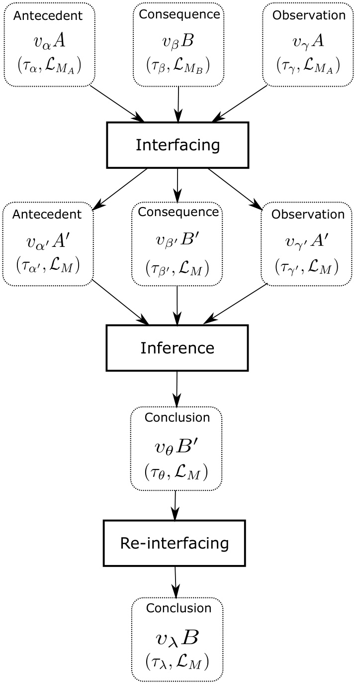
Figure 2.
Inference with multi-bases multi-sets
4.1. Interfacing of manipulated multi-sets
The aim of this stage is to translate the manipulated multi-sets of the GMP schema (those of the antecedent, the consequence, and the observation) to a unique base . However, this conversion to the new base must guarantee non-information loss. For that, we propose to calculate the base size M using the least common multiple (LCM) [33] of the different base sizes and . We subtract 1 from every base size because the numeration of degrees in a multi-valued base starts with 0. The size of the new common base is obtained as follows:
With the use of LCM, every degree from or will have its corresponding degree in the base . For example, having the bases and , the common base size is . Figure 3 illustrates visually this example. We can see that the degree of the base is equivalent to the degree in the base , and of the base is equivalent to in the base , and so on.
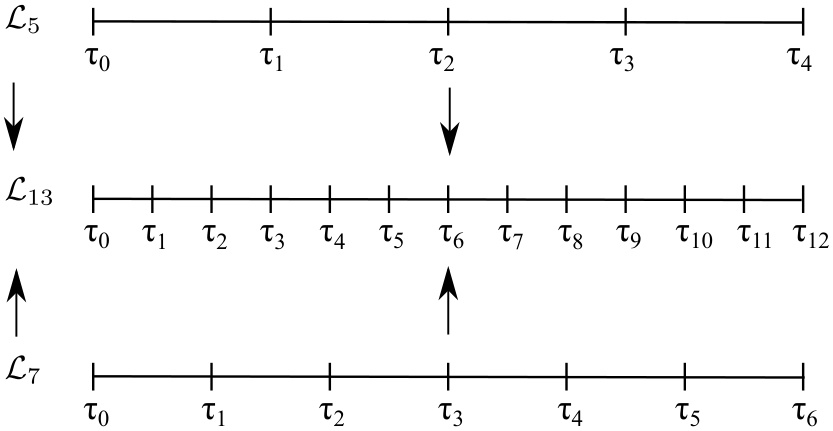
Figure 3.
Example of determination of the common base with LCM
The multi-sets , , and must then be translated to the common base . To do that, we propose to apply a linguistic modifier to the considered multi-sets. To avoid information loss, this linguistic modifier must conserve their proportions. This will guarantee that the notion expressed by a multi-set will not be modified. So the mode of this linguistic modifier must be central (see section 2.2.). Moreover, the linguistic modifier must change the base to become . The new base size M is in all cases a multiple of the base size of the multi-set (subtracted by 1), since it is a LCM of all base sizes. The nature of the linguistic modifier is consequently dilation. As mentioned in the table 1, the modifier that conserves the proportion and increases the base size is DC (Dilating Central). We conclude that the linguistic modifier that we will use in the translation is DC. Let us recall its definition:
The modifier DC changes the degree to , and changes the base size to . So it acts as a zoom in by multiplying the degree and the base size by (with subtracting it by 1 for the base size).
It remains to determine the radius of the modifier DC for the interfacing, which represents its intensity. Suppose that we would translate the proposition into the base . The operator DC transforms a base to its multiple. Moreover, the intended base is a multiple of since it is its LCM. So the ratio of DC must be . This ratio will also be used for the conversion of since they have the same base. In the same way, the ratio of the conversion for the proposition will be . If we return to the example of figure 3, to translate the degree of the base to the base , the used modifier is . This will give the new multi-set: .
4.2. Symbolic inference
Having all the multi-sets on the same base , we can apply our approximate reasoning (10). So, the GMP (12) on the base becomes the following:
The degree of the inference conclusion is determined using The GMP (10). Thus, it is obtained by the following formula:
4.3. Re-interfacing of the result
The obtained inference conclusion in the previous stage is on the common base . It is then necessary to give it back to the base . For that, we propose to also do that with a linguistic modifier. This modifier should conserve the proportion of the multi-set to avoid information loss, so it must be central. Moreover, it will change the base size M of the intermediate result to . More precisely, it will decrease the base size, since the base is a LCM of the targeted base . For that, the nature of the used linguistic modifier should be erosion. Consequently, we conclude that the used modifier for the re-interfacing is EC (Eroded Central) (see table 1). Its definition is the following:
Here, with this modifier, the degree and the base size are divided by . Thus, it acts like a zoom out of the multi-sets. The obtained degree and base size after the modification are the dividers of the original ones.
The problem that then arises is to determine the radius of the modifier EC. The radius represents its intensity. It must lead the intermediate conclusion, which is in the base , to its original base, which is . As is the LCM of , is a divider of . So the ratio of EC must be . Consequently, the degree of the final conclusion is obtained by the following formula:
For example, if the intermediate result is the degree in the base (see fig. 3), its re-interfacing to the base gives . So the deduced degree is in the base .
4.4. Summary form of the method
We summarize in the proposition 1 the procedure to determine the inference conclusion from the inference schema (12) where the multi-sets A and B have different bases.
Proposition 1.
Given the multi-sets A and B of the bases and respectively. With a rule and an observation of the form:
- “If X is then Y is ”
- “X is ”
we can conclude that “Y is ” with: ,
where and .
Example 2.
Consider the bases and with the following scales:
{not-at-all, very-little, little, somewhat, moderately, more or less, enough, very, completely}
{not-at-all, very-little, little, moderately, enough, very, completely}
The multi-sets pale and blood flow are associated to the bases and respectively. With the following data, we obtain this result:
We calculate first the base size M:
The intermediate conclusion is determined as follows:
Then we deduce that:
This corresponds to the linguistic degree moderately in the scale .
If we try the same method with another observation, we obtain:
The degree is determined as follows:
We conclude that the rank degree of the final result is:
This corresponds to the linguistic degree enough in the scale .
5. Consideration of complex rules
The approximate reasoning that we proposed in the previous section is a simplified form of what we can find in rule-based systems. It handles a simple rule whose antecedent and consequence are composed of a unique proposition each. In practice, rule-based systems contain rules whose premise and conclusion can be a conjunction or a disjunction of propositions, or combinations of them. We discuss in this section these cases, and we specify how to infer with them. We will suppose here that all the manipulated multi-sets have the same base. The multi-bases problem is examined in the next section.
5.1. Conjunctive rules
A conjunctive rule has a premise that is a conjunction of propositions. To infer with such a rule, the observation must also be a conjunction of propositions whose predicates are the same as those of the premise. Thus, the reasoning schema becomes the following:
The problem is how to evaluate the transformation between the premise and the observation, and how to translate it in order to calculate the degree of the inference conclusion. In other words, how can the term and be mathematically modeled to calculate the degree ?
In fuzzy logic, the term and is generally formalized by a fuzzy connective [34,35,36,37]. We say that a binary operation f is a fuzzy connective if it verifies the following axioms:
- f gives the same results of the classical logic connectives and when the degrees are precise and certain;
- f is commutative, monotone and associative.
These properties are verified by T-norms and T-conorms. For simplicity reasons, fuzzy community generally uses the operators min and max as fuzzy connectives to replace, respectively, and in fuzzy context.
We choose in this work to consider min and max as symbolic multi-valued connectives. We note them respectively by and as for classical logic. So, for the case of conjunctive rules, the principle of our solution is to aggregate by the connective the different transformations between every couple of propositions from the premise and the observation that have the same predicate.
Proposition 2.
Given a rule and an observation of the form:
- “If is and …and is then Y is ”
- “ is and …and is ”
Example 3.
Having the scale base , the following rule and fact allow deducing that:
We use the Łukasiewicz T-norm (4) and implication operator (6) to determine the conclusion by the proposition 2:
Which allows determining the following:
The symbolic degree corresponds to the term “little” from the base , so the conclusion is: “Malaria is little severe”.
And if we consider the following data we can deduce:
The degree of the conclusion is determined as follows:
The resulted degree is:
The symbolic degree corresponds to the term “enough”, so the conclusion is: “Malaria is enough severe”.
As we can see in the example, our approximate reasoning with the conjunctive rule has the same behavior as the simple rule. Indeed, we remark that if the propositions of the observation are a weakening of the propositions of the rule premise, then the inference conclusion is a weakening of the rule conclusion. Otherwise, the inference conclusion obtains the same value as the rule conclusion. This corresponds to our expectations in order to verify the criterion II-2 of the axiomatics (2).
5.2. Disjunctive rules
A disjunctive rule is a rule whose premise is a disjunction of propositions. The disjunction is formulated by the term or between propositions. The Generalized Modus Ponens with such a rule is the following:
As for the conjunction case, the aim is to aggregate the transformation between the propositions of the premise and of the conclusion. We consider for that the connective .
Proposition 3.
Given a rule and an observation of the form:
- “If is or …or is then Y is ”
- “ is or …or is ”
where and B are multi-sets on the base . We can deduce that “Y is ” with:
Example 4.
Having the list of truth-degrees , with the following knowledge we conclude:
One obtains the conclusion with proposition 3 as follows:
We can then determine the inferred degree:
The determined degree represents the term “moderately” in the scale base . So, the deducted conclusion is: “Malaria is moderately severe”.
6. Reasoning with multi-bases knowledge and complex rules
After treating the presence of multi-bases multi-sets and complex rules separately, we consider in this section the presence of multi-bases multi-sets and complex rules in the same inference model. We consider in this section the case where the antecedent is a conjunction of propositions, which is the more used form. When a rule is disjunctive (the premise is with OR connective), the same procedure and formulas can be adopted. Just must replace the connective by , and it will be modeled by the max operator instead of the min operator.
For the conjunctive rule, the observation must also be composed by a conjunction of propositions whose predicates are the same as that of the antecedent. Approximate reasoning in this case is formalized by the following schema:
with and B are multi-sets. In this situation, these multi-sets have different bases, which we denote by and respectively.In order to infer with these knowledge, we propose to follow the same principle as the reasoning with multi-bases multi-sets described in Section 4., while aggregating the imprecision of the composed rule premise and the composed observation as explained in Section 5.. Consequently, tree stages are necessary, which are: interfacing of manipulated multi-sets; inference; and re-interfacing of the result.
6.1. Interfacing of manipulated multi-sets
The interfacing of the multi-sets consists of translating them to a common base . The size M of this base is obtained by the Lower Common Multiple of all the base sizes that appear in the GMP (21), which are and . Thus, it is determined by the following formula:
The conversion of the considered multi-sets to the base is made by the modifier DC (Dilating Central in table 1). Indeed, this modifier will dilate their bases in order to reach the base size M. Every multi-set will have its own radius according to its base size. The radius of the modification will be, for every multi-set, divided by the base size of the multi-set minus one. So for a multi-set , , the value of the radius is , and for B it is .
6.2. Symbolic inference
Once all the multi-sets are on the same base, approximate reasoning can be executed. This will determine a new assertion from the following schema:
Here, the multi-set is the equivalent of the multi-set B on the base . The problem encountered here is the consideration of complex rules in the inference process. The challenge is how to aggregate the imprecision of the whole antecedent and the observation to consider it in the determination of the inference conclusion. We already proposed in Section 5. a solution to reason with complex rule in the case of mono-base (see proposition 2). This reasoning model can be used here since all the manipulated multi-sets have the same base. Consequently, the resulted degree of the inference after interfacing is obtained as follows:
6.3. Re-interfacing of the result
The obtained result in the previous step is on the base . It is then necessary to translate it under the conclusion base , as it is imposed by the expert. In order to do that, we propose to use the modifier EC (Eroded Central) as for the simple inference schema described in Section 4.. This modifier will erode the base of the multi-set by dividing its size M until reaching the desired base size . Consequently, and using the definition of EC (see table 1), the degree of the inference conclusion is obtained as follows:
6.4. Summary of the method
We present below a proposition that summarizes the procedure to determine a conclusion in the presence of a conjunctive rule and multi-bases multi-sets.
Proposition 4.
Given a conjunctive rule and an observation of the form:
- “If is and …and is then Y is ”
- “ is and …and is ”
where and B are multi-sets of the bases and . We can conclude that “ Y is ” with:
where andIn the same way, when the rule is disjunctive instead of conjunctive, the conclusion of the inference is obtained by following the proposition 4 with replacing by .
Example 5.
Having the lists of truth-degrees:
{not-at-all, very-little, little, somewhat, moderately, more or less, enough, very, completely},
{not-at-all, very-little, little, moderately, enough, very, completely},
{not-at-all, little, moderately, enough, completely},
and the multi-sets pale, numb and low in the basis , and respectively. The following rule and observation give as result:
The conclusion degree of the inference with these data are obtained by calculating first the base size:
The intermediate conclusion is determined as follows:
So, the degree of the final conclusion is:
This corresponds to the linguistic degree moderately in the scale .
If the input is the following, we obtain:
The intermediate conclusion is determined as follows:
So, the degree of the final conclusion is calculated as follows:
This corresponds to the linguistic degree enough in the scale .
7. Discussion
The proposition 4 allows inferring with both multi-bases multi-sets and conjunctive rules. Thus, the determination of the conclusion by the proposition 4 generalizes that of the proposition 1 when the number n of propositions in the rule antecedent is equal to 1. Also, it generalizes that of the proposition 2 when the base sizes ( ) and are equal. Moreover, the determination of the conclusion by the proposition 1 generalizes that of the Generalized Modus Ponens (10) which considers a simple rule when A and B have the same base. We deduce that the proposition 4 gives a general form for our cautious approximate reasoning.
In a rule-based system, considering data imprecision can be performed by integrating this approximate reasoning into its inference engine. The purpose of the inference engine in rule-based systems is to simulate a human deduction based on a set of facts and a set of rules. Its principle is to enchain cycles, each comprising approximate reasoning phase in order to consider rule chaining. A multi-set can be present in more than one rule consequence. For that, it is necessary to make combination of conclusions. This can be made by the max operator, as in fuzzy rule-based systems.
As we mentioned before, the particularity of this approximate reasoning compared to other approaches of approximate reasoning is that it gives a conclusion equal to the rule consequence when the observation is a reinforcement of the rule antecedent. It is then useful for specific rules whose antecedent and consequence do not have a big causality and do not then require gradual reasoning. Its use must be decided by the domain expert. Indeed, he knows the characteristics of the knowledge in the antecedent and the consequence of every rule, as well as their causality relation. This leads to realize that in the same rule-based system, we may have to define rules which do not necessarily have the same behavior. For that, we propose to associate with each defined rule in the rule-based system a parameter to specify the behavior of the rule in order to know which approximate reasoning will be used for this rule: gradual reasoning (type 1) or cautious reasoning (type 2).
8. Conclusion
In this paper, we focused on the approximate reasoning based on implication operator that is proposed in the multi-valued context [21]. We gave proofs that this model checks the axiomatics of approximate reasoning defined in the literature. This approximate reasoning nevertheless considers multi-sets having the same base. Moreover, it infers only with a simple fact and a simple rule, whose premise and conclusion consist each of a single proposition. For that, we considered other types of knowledge in the inference process. We improved this approximate reasoning to handle multi-bases multi-sets. Moreover, we treated the case of complex rules, where the premise is a conjunction or a disjunction of propositions. We finally proposed a general form of cautious approximate reasoning that generalizes all the treated cases in the paper. A perspective of this work is to build a multi-valued rule-based system that integrates our two types of approximate reasoning.