

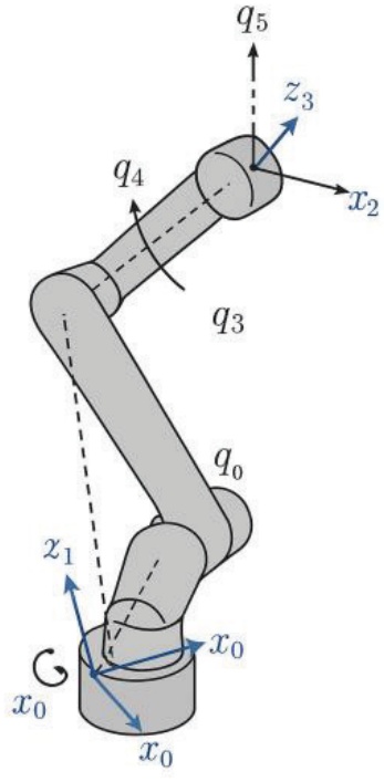
Figure 1.
Kinematic models of a UR5e robot using DH parameters
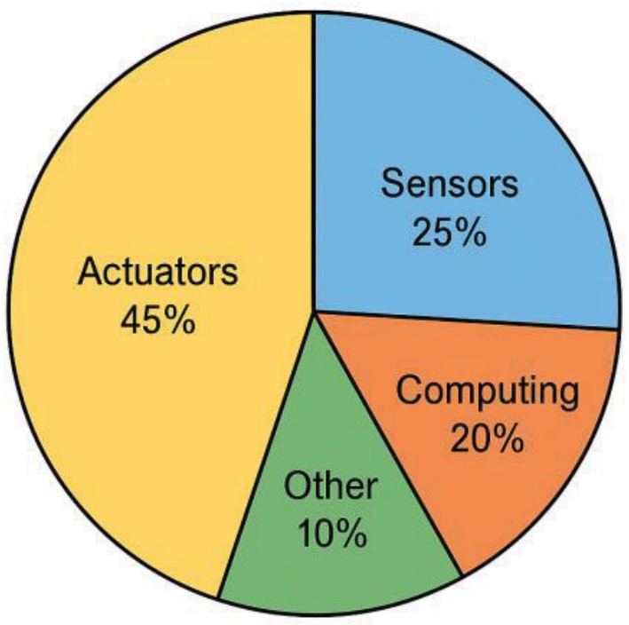
Figure 2.
Energy consumption breakdown of a collaborative robot
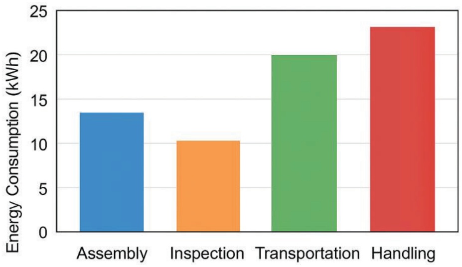
Figure 3.
Energy consumption comparisons of different robotic operations
Table 1.
Assumptions in energy modeling of collaborative robots
| Sr. No. | Parameter | Symbol / Unit | Assumed Value | Description |
|---|---|---|---|---|
| 1 | Supply Voltage | Vs (V) | 24 V | Standard voltage for robot actuators and sensors |
| 2 | Motor Efficiency | ηm (%) | 85% | Efficiency of DC or servo motors driving actuators |
| 3 | Control System Efficiency | ηc (%) | 90% | Power conversion and control losses considered |
| 4 | Sensor Power Consumption | Ps (W) | 25 W | Average power required by vision and proximity sensors |
| 5 | Computing Load Power | Pc (W) | 20 W | Energy used for onboard data processing and control |
| 6 | Idle Power Consumption | Pi (W) | 5 W | Baseline power consumption when robot is in standby mode |
| 7 | Duty Cycle | Dc (%) | 70% | Active operation percentage during task cycle |
| 8 | Ambient Temperature | Ta (°C) | 25 °C | Normal laboratory working conditions |
| 9 | Energy Recovery Efficiency | ηr (%) | 10% | Portion of kinetic energy recovered during braking or deceleration |
Table 2.
Metrics to evaluate the optimization outcomes
| Sr. No. | Metric | Description | Unit |
|---|---|---|---|
| 1 | Total Energy (J) | Integral of actuator power | Joules |
| 2 | Task Time (T) | Duration of trajectory | Seconds |
| 3 | Smoothness | Mean-squared jerk | m2/s5 |
| 4 | Optimization Time | Algorithm runtime | Seconds |
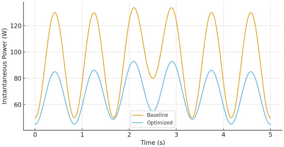
Figure 4.
Energy consumption profile — baseline vs. optimized trajectory
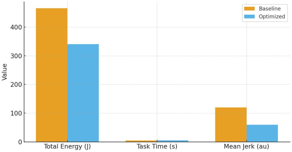
Figure 5.
Performance metrics— baseline vs. optimized
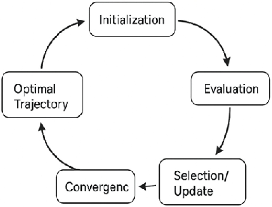
Figure 6.
Generic workflow of intelligent optimization algorithms
Table 3.
Comparison of Optimization Algorithms for Robot Energy Efficiency
| Sr. No. | Algorithm | Strengths | Limitations | Suitable Application |
|---|---|---|---|---|
| 1 | PSO | Fast convergence, easy implementation | May stagnate in local minima | Continuous trajectory optimization |
| 2 | GA | Strong global search, flexible encoding | Computationally heavy | Complex multi-variable problems |
| 3 | RL | Adaptive, model-free learning | Requires extensive training data | Dynamic, uncertain environments |
Table 4.
Algorithm setting
| Sr. No. | Algorithm | Population Size | Iterations | Learning Rate / Crossover Prob. | Convergence Criterion |
|---|---|---|---|---|---|
| 1 | PSO | 30 | 100 | 0.7 (inertia w) | ΔE < 1 × 10⁻³ J |
| 2 | GA | 50 | 150 | 0.8 (crossover) / 0.05 (mutation) | Fitness change < 0.01 % |
| 3 | RL (Q-Learning) | — | 500 episodes | α = 0.1, γ = 0.9 | Average reward > 0.95 Rmax |
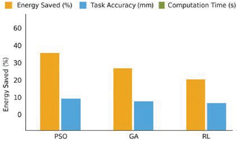
Figure 7.
Performance comparison of optimization algorithms
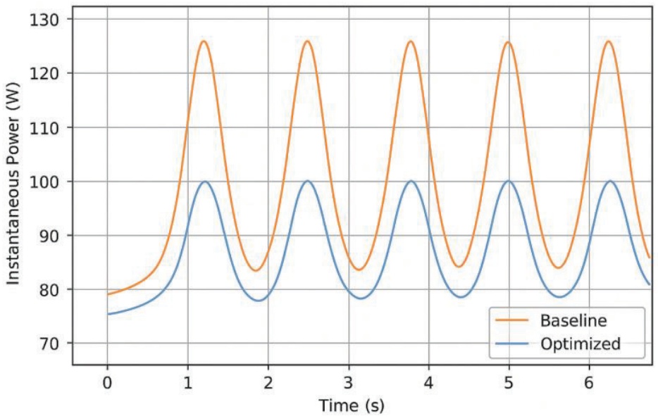
Figure 8.
Energy consumption profile — baseline vs. optimized
Table 5.
Energy Consumption and Task Efficiency Comparison
| Sr. No. | Algorithm | Total Energy (J) | Reduction (%) | Task Time (s) | Mean Jerk (m2/s5) |
|---|---|---|---|---|---|
| 1 | Baseline | 480 | — | 7.2 | 1.25×10⁴ |
| 2 | PSO | 340 | 29 | 7.1 | 8.5×10³ |
| 3 | GA | 375 | 22 | 7.4 | 9.2×10³ |
| 4 | RL | 360 | 25 | 7.0 | 7.8×10³ |
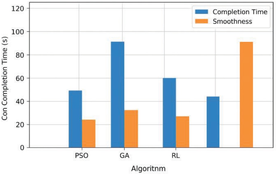
Figure 9.
Task completion time and smoothness comparison
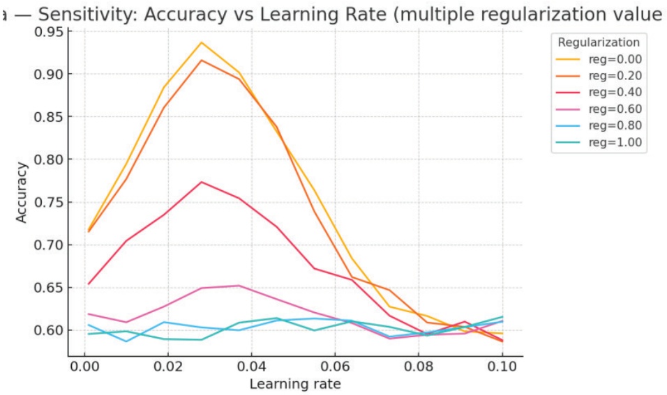
Figure 10.
Sensitivity analysis — effect of algorithm parameters