

Table 1.
Comparison of Precision Farming and Conventional Farming Practices
| Feature | Precision Farming | Conventional Farming |
|---|---|---|
| Efficiency | Increased efficiency through tech | Lower efficiency |
| Resource Conservation | Minimizes resource overuse | Resource-intensive |
| Data-Driven Decision-Making | Informed decisions through data analysis | Experience-based decisions |
| Labor Requirements | Reduced labor needs (automation) | Labor-intensive |
| Environmental Impact | Reduced environmental impact | Environmental concerns |
| Initial Costs | Higher initial costs | Lower initial costs |
| Complexity | Complex data management | Simplicity and familiarity |
| Sustainability | Enhanced sustainability | Reduced sustainability |
Table 2.
Open Data Resources in the Field of Smart Agriculture [6]
| Data Source | Description |
|---|---|
| USDA National Agricultural Statistics Service (NASS) Data | Crop production, livestock statistics, and agricultural information in the United States |
| European Space Agency’s Sentinel Data | High-resolution satellite imagery for crop monitoring and land use |
| NOAA Climate Data | Weather and climate data, including forecasts, rainfall, and temperature |
| Global Open Data for Agriculture and Nutrition (GODAN) | Open datasets related to agriculture, food security, and nutrition |
| NASA Earthdata | Remote sensing data for monitoring climate, soil moisture, and vegetation |
| FAO Data | Agricultural data and information on global food production and trade |
| IoT Sensor Data | Sensor data, such as soil moisture and temperature, from IoT devices in fields |
| Crop and Soil Databases | Information on crop yields, soil quality, and nutrient levels |
| Agricultural Research Institutions | Data from research institutions on crop trials, pest monitoring, and experiments |
| OpenWeatherMap | Weather data, including current conditions, forecasts, and historical records |
| Government Agricultural Portals | Information on farming practices, subsidies, and agricultural policies |
| Community-Generated Data | User-generated data sharing experiences, practices, and insights |
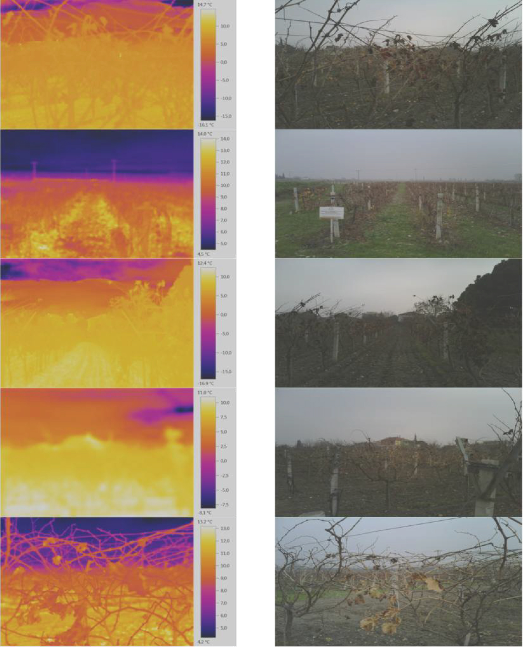
Figure 1.
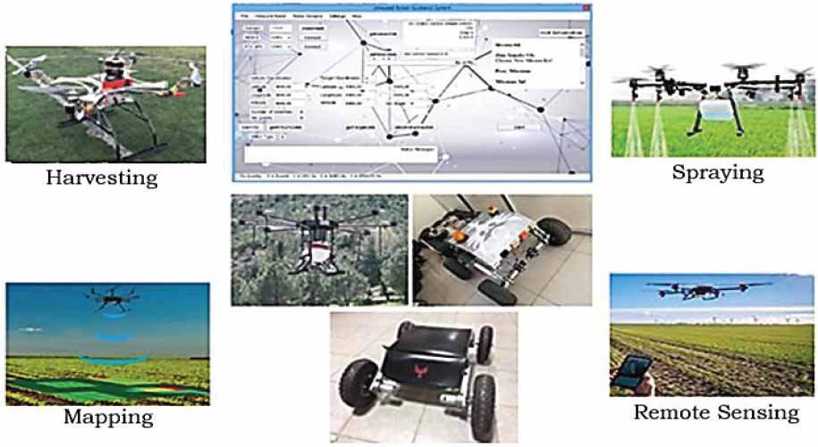
Figure 2.
Table 3.
Comparison of UAVs and UGVs in Agricultural Farm Operations
| Feature | UAVs (Unmanned Aerial Vehicles) | UGVs (Unmanned Ground Vehicles) |
|---|---|---|
| Mobility | Operate in the air, offering a bird’s-eye view ofthe entire field. | Operate on the ground, moving at ground level and typically covering less area. |
| Data Collection | Useful for aerial imaging, crop monitoring, and capturing visual and multispectral data. | Suited for close-up inspections, soil sampling, and carrying sensors at ground level. |
| Field Coverage | Can cover large areas efficiently and quickly, making them ideal for large farms. | Better for smaller, precision tasks and for navigating through tighter spaces. |
| Real-time Monitoring | Can provide real-time data and immediate insights from above. | May require additional data processing or time to convey ground-level information. |
| Accessibility | Easily access difficult-to-reach areas and fields with various terrains. | Limited by obstacles and may face challenges on uneven terrain. |
| Crop Health Assessment | Efficient for monitoring crop health, identifying stress, and assessing overall field conditions. | Useful for proximity analysis, detecting plant diseases, and assessing soil quality. |
| Data Accuracy | Offers high-resolution imaging and data collection capabilities, especially with advanced sensors. | May have limitations in capturing high-resolution data, depending on the UGV’s setup. |
| Cost | UAVs can be more cost-effective for large-scale surveillance of vast areas. | UGVs can be cost-effective for specific, targeted tasks and smaller plots. |
| Versatility | Well-suited for scouting and monitoring tasks but not for physical intervention or soil manipulation. | Can perform tasks like weeding, planting, and soil sampling directly. |
| Limitations | Affected by weather conditions and regulations related to airspace. | Constrained by the limitations of ground mobility and potential obstacles. |
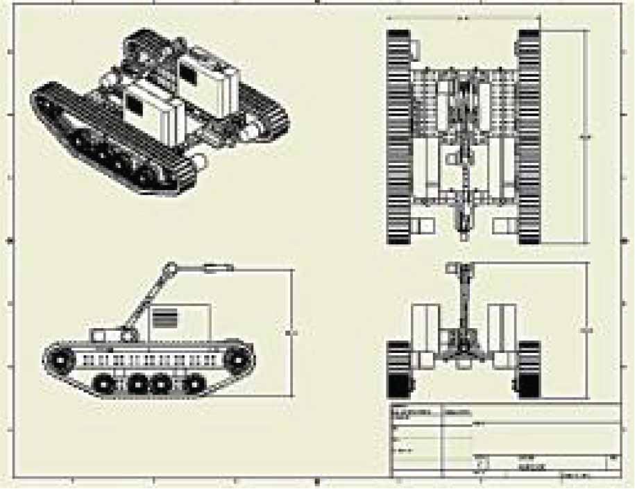
Figure 3.
Design of the Tracked Robot Platform
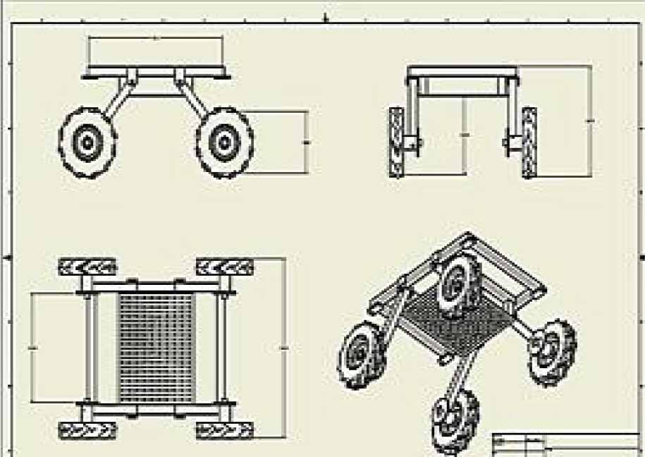
Figure 4.
Isometric and Three-Dimensional View of the Wheeled Robot Platform
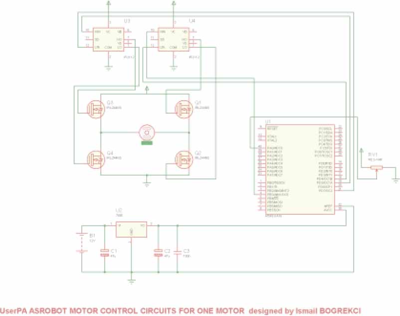
Figure 5.
Circuit for Motor Control
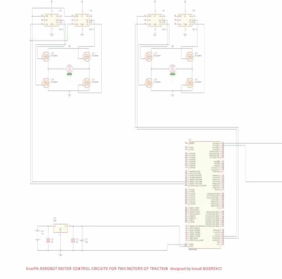
Figure 6.
Circuit for Controlling Two Motors for Locomotion
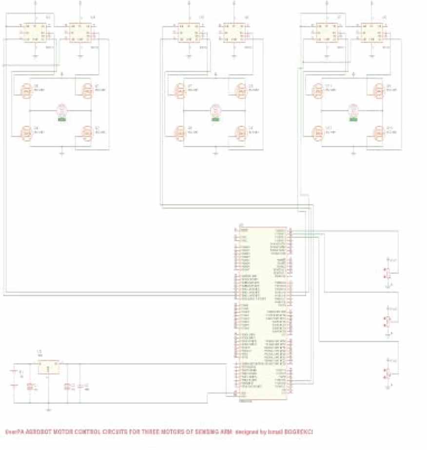
Figure 7.
Circuit for Controlling Two Motors for Locomotion
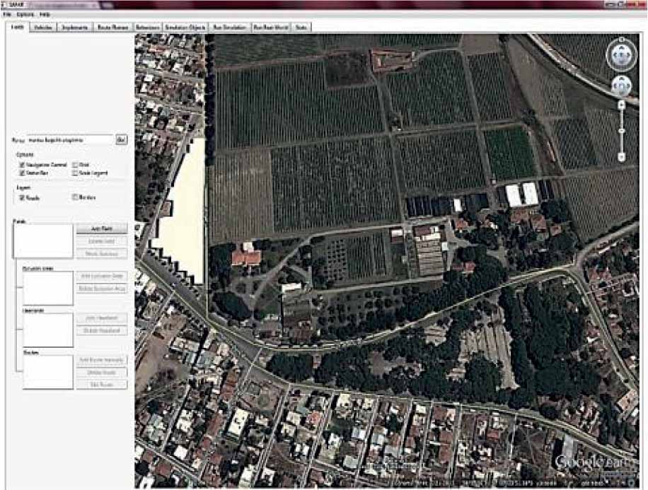
Figure 8.
Determination of Agricultural Land [Safar]
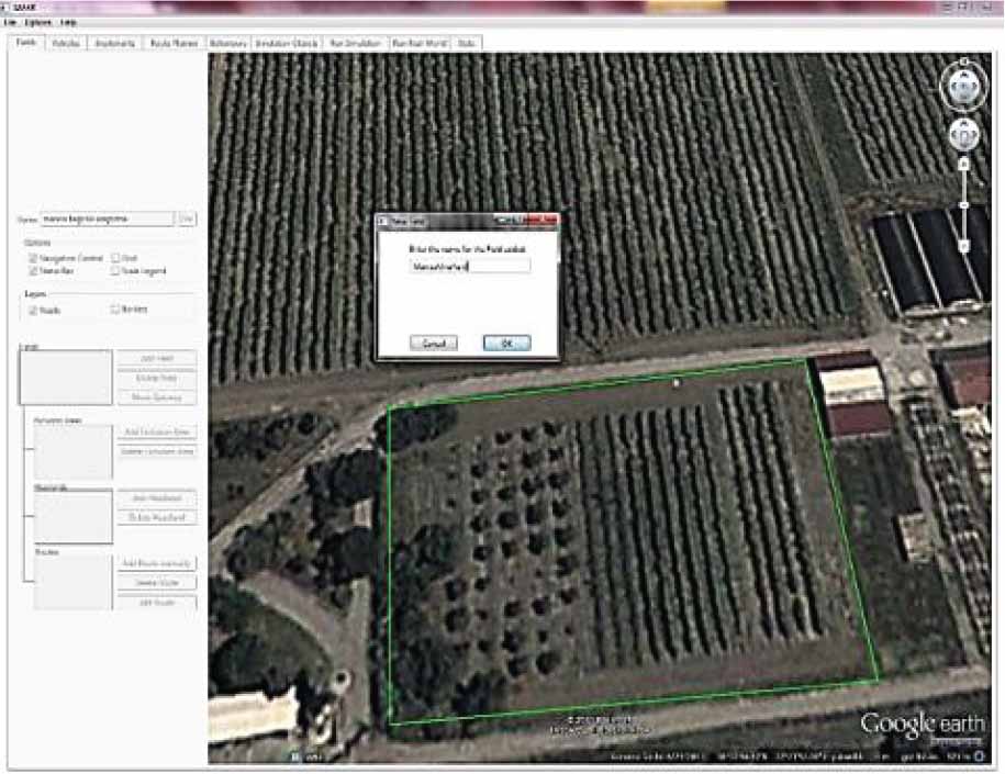
Figure 9.
Drawing and Defining Field Boundaries [Safar]
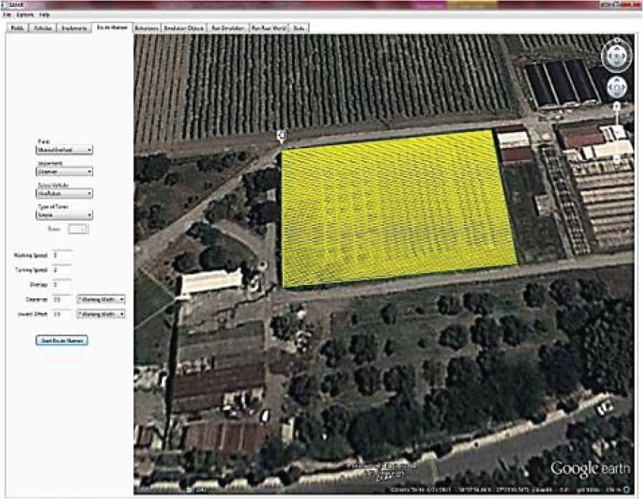
Figure 10.
Determination of the Route, Adding Robots and Equipment [Safar]
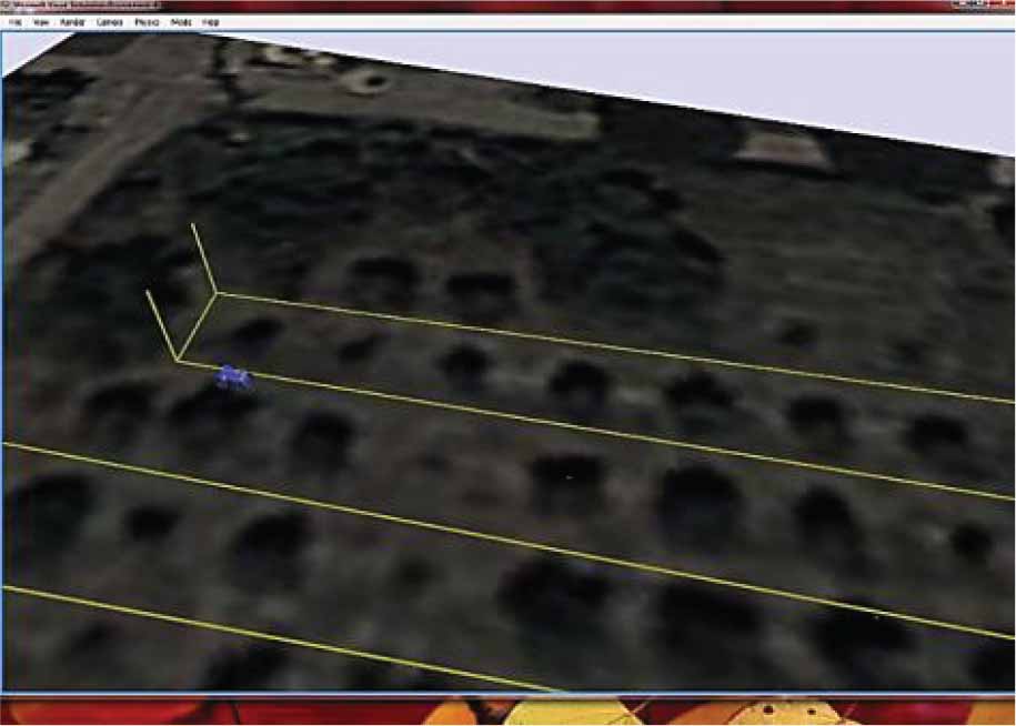
Figure 11.
Running the Simulation [Safar]
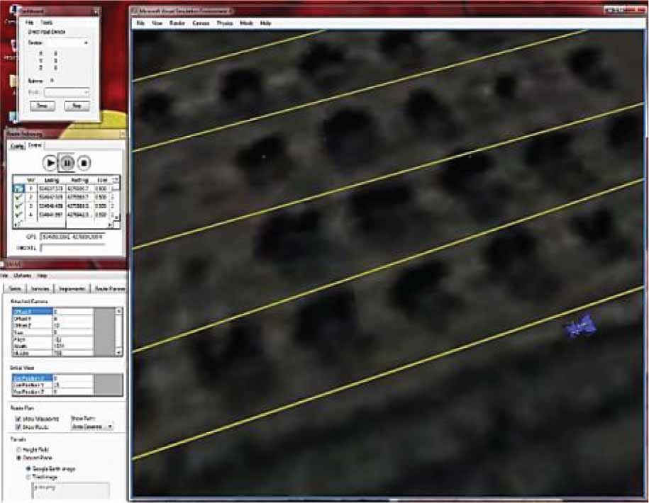
Figure 12.
System Operation Through Integration [Safar]
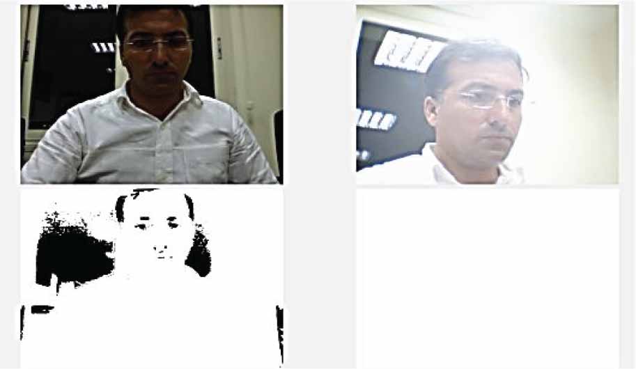
Figure 13.
Office-Based Testing of Distance Measurement Using Stereo Imaging
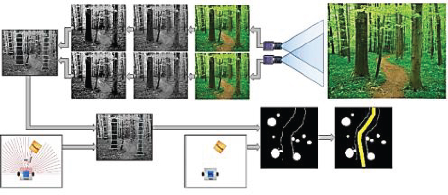
Figure 14.
Results of Topography Determination Using Stereo Imaging Studies
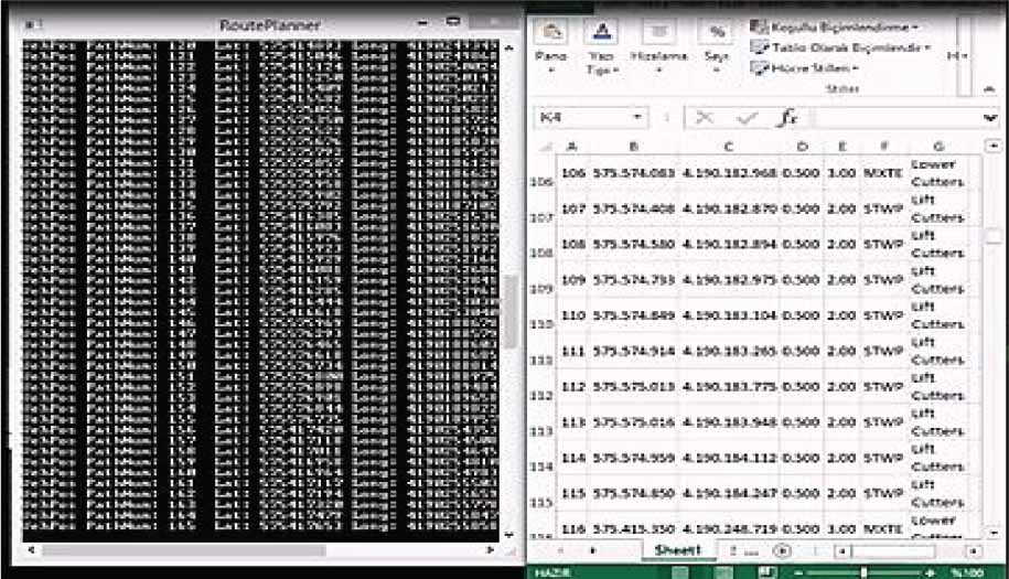
Figure 15.
RTK-GPS Route Determination and Planning Study
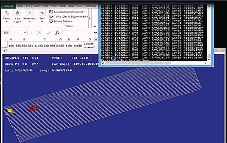
Figure 16.
Simulation of Robot Maneuvering on RTK-GPS Route Determination and Planning
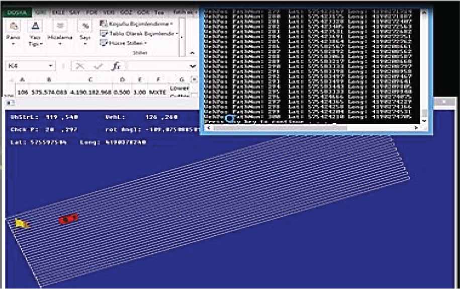
Figure 17.
Simulation of Robot Maneuvering on RTK-GPS Route Determination and Planning - Route Numbers
Table 4.
Comparison of UAVs and UGVs in Agricultural Farm Operations
| Machine Learning Model | Use Case in Agro-Ecosystems |
|---|---|
| Linear Regression | Crop yield prediction, soil quality assessment |
| Decision Trees | Pest detection, crop disease identification |
| Random Forest | Crop classification, yield forecasting |
| Support Vector Machines | Weed detection, precision agriculture |
| Neural Networks | Weather forecasting, crop monitoring, yield prediction |
| K-Nearest Neighbors | Soil health assessment, precision agriculture |
| Naive Bayes | Disease risk assessment, crop disease identification |
| Clustering (K-Means) | Crop grouping, yield pattern analysis |
| Principal Component Analysis (PCA) | Dimensionality reduction for feature extraction |
| Long Short-Term Memory (LSTM) | Time-series data analysis, weather prediction |
| Convolutional Neural Networks (CNN) | Image-based pest and disease detection |
| Reinforcement Learning | Autonomous farming, autonomous machinery control |
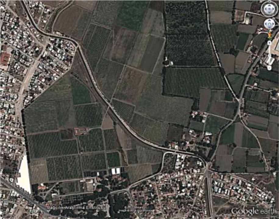
Figure 18.
Location Images of the Manisa Viticulture Research Station
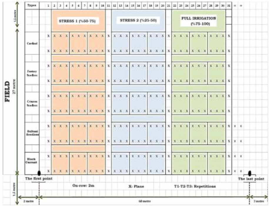
Figure 19.
Experimental Design
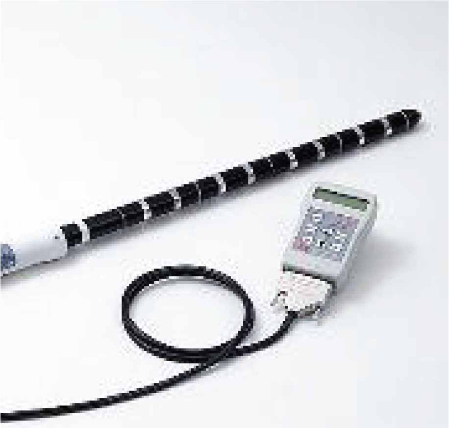
Figure 20.
Profile Probe
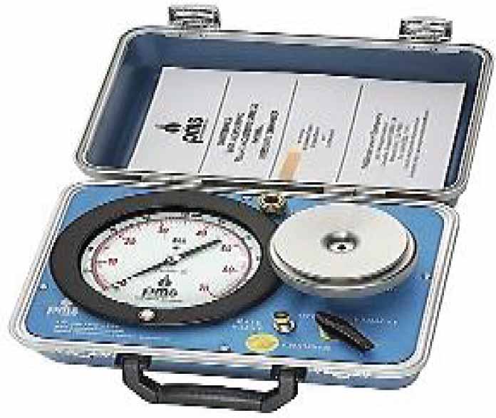
Figure 21.
A portable Scholander Pressure Chamber
Table 5.
Comparison of UAVs and UGVs in Agricultural Farm Operations
| Depth (cm) | Saturation (%) | Texture | Total Salinity (%) | PH | CaCO3(%) | Total N (%) |
|---|---|---|---|---|---|---|
| 0–30 | 30.00 | Sandy | 0.0113 | 7.80 | 5.60 | 0.11 |
| 30–60 | 31.00 | Loamy | 0.0159 | 7.87 | 4.80 | 0.11 |
| 60–90 | 37.00 | Loamy | 0.0282 | 7.88 | 8.00 | 0.09 |
| Condition | Non-Saline | Slightly Alkaline | High | Medium | ||
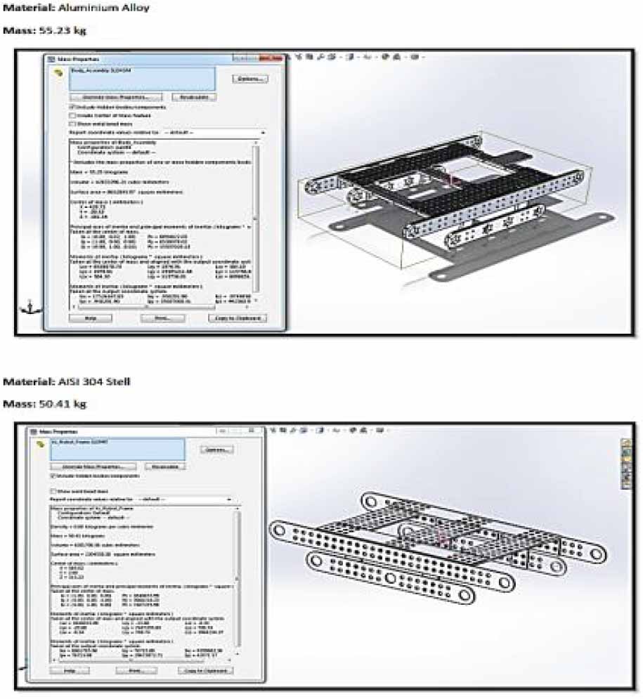
Figure 22.
The design of the robot platform, its center of gravity, and dimensional specifications
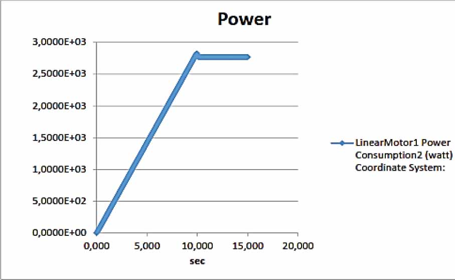
Figure 23.
Dynamical Simulation Results of the Robot (Power)
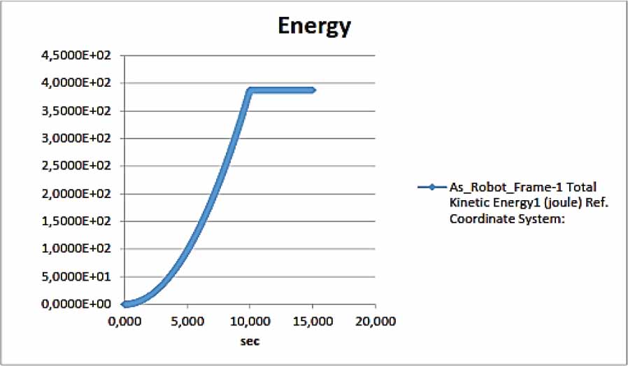
Figure 24.
Dynamical Simulation Results of the Robot (Energy)
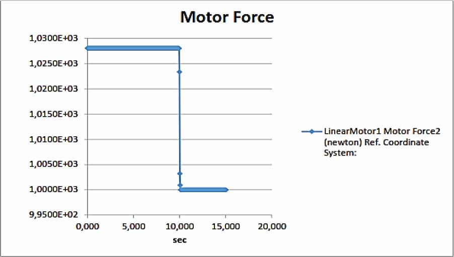
Figure 25.
Dynamical Simulation Results of the Robot (Motor Force)
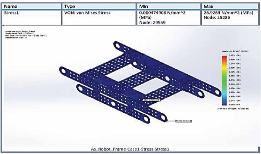
Figure 26.
Static Analysis Results of the Robot (Stress)
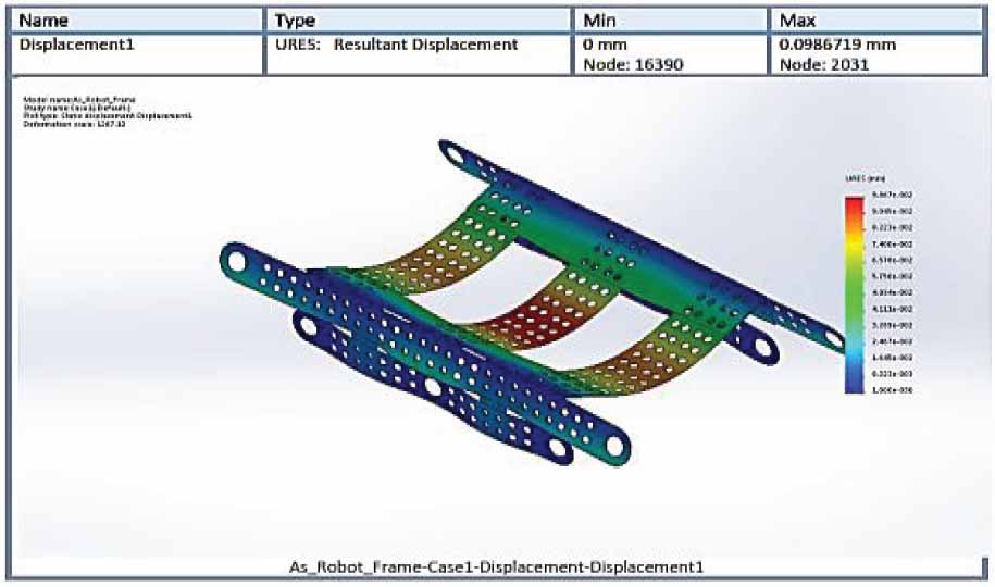
Figure 27.
Static Analysis Results of the Robot (Displacement)
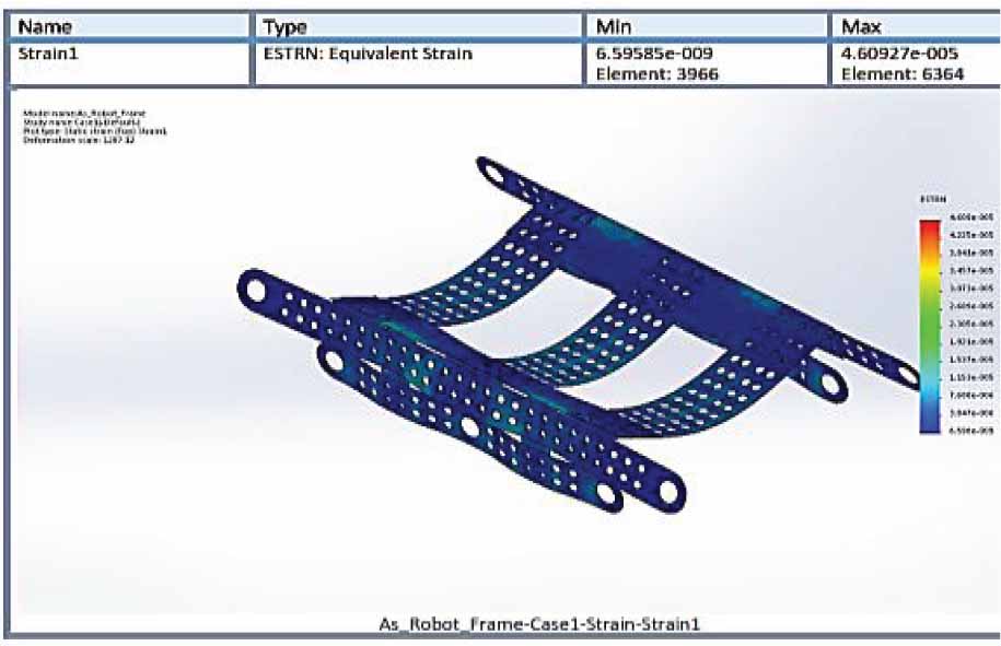
Figure 28.
Static Analysis Results of the Robot (Strain)
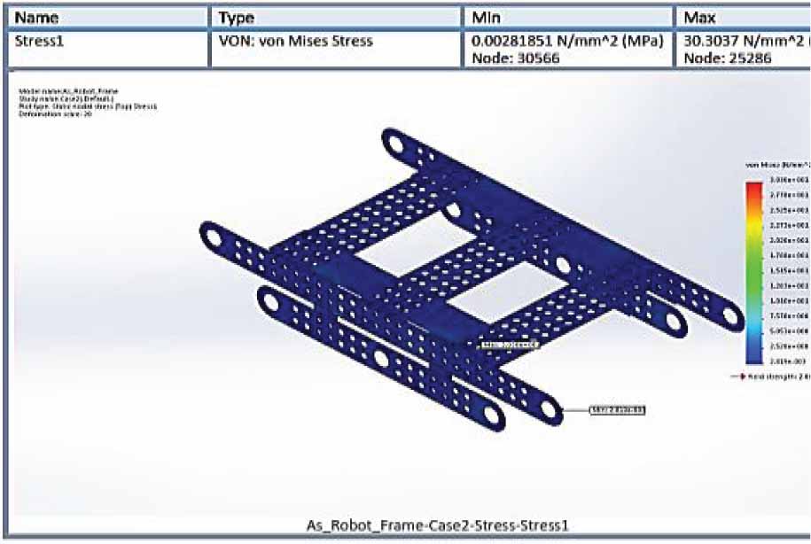
Figure 29.
Dynamic Analysis Results of the Robot (Stress)
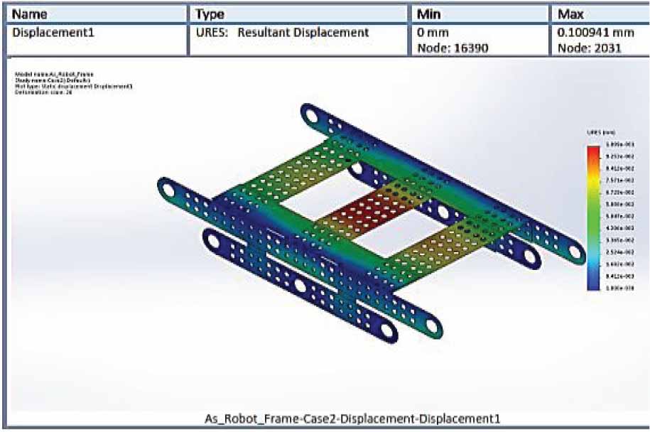
Figure 30.
Dynamic Analysis Results of the Robot (Displacement)
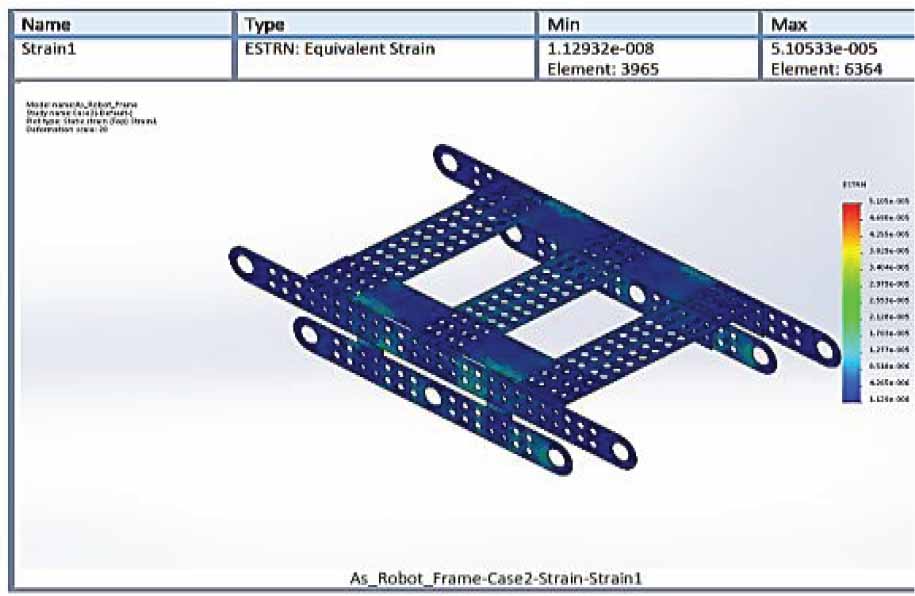
Figure 31.
Dynamic Analysis Results of the Robot (Strain)
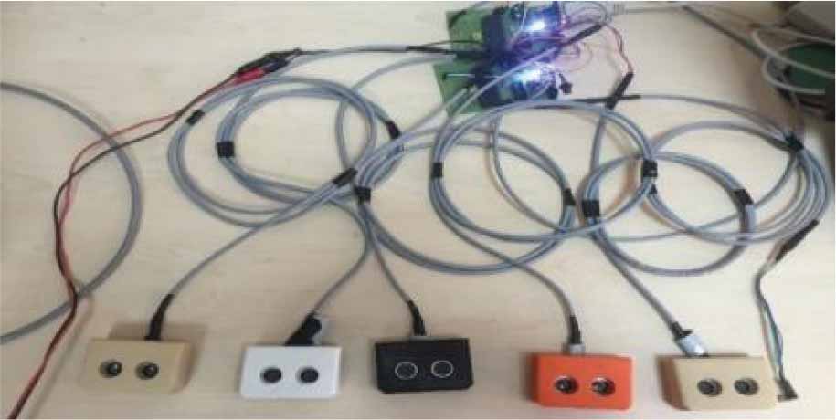
Figure 32.
The version operated with improved detection cards for calipers and ultrasonic sensors
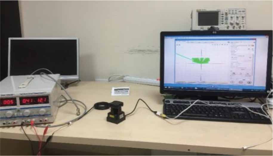
Figure 33.
LIDAR detectino
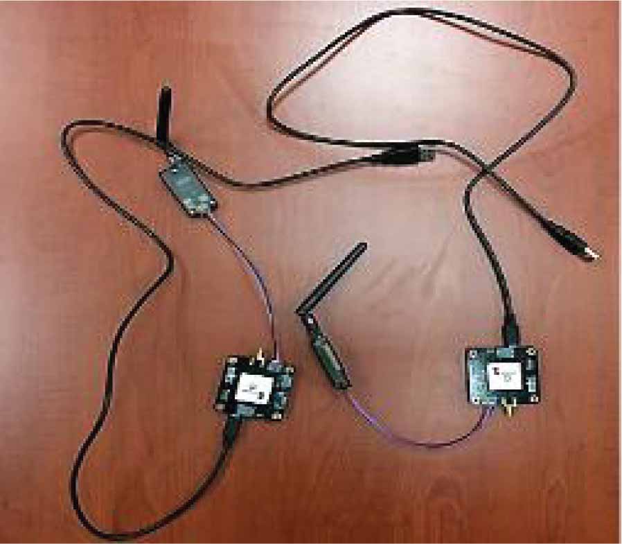
Figure 34.
RTK-GPS to be used for guiding the robot
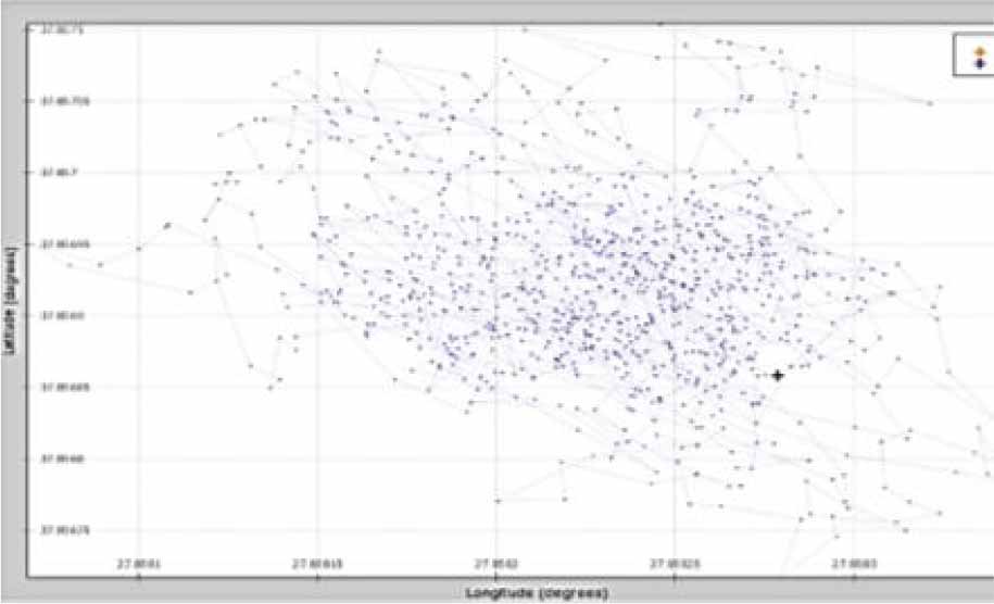
Figure 35.
The Standard GPS SPP graph
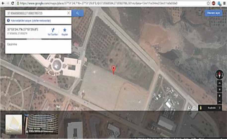
Figure 36.
Google Maps output (37°51’24.7”N 27°51’29.8”E 37.856858, 27.858279)
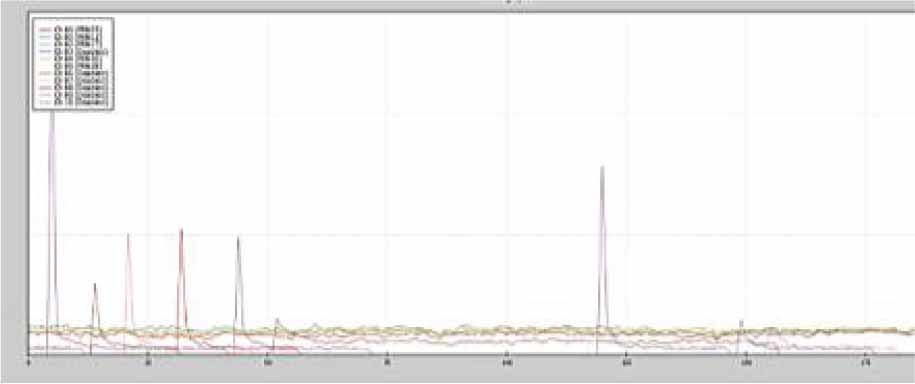
Figure 37.
Tracking Screen
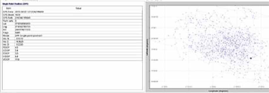
Figure 38.
Analysis Screen
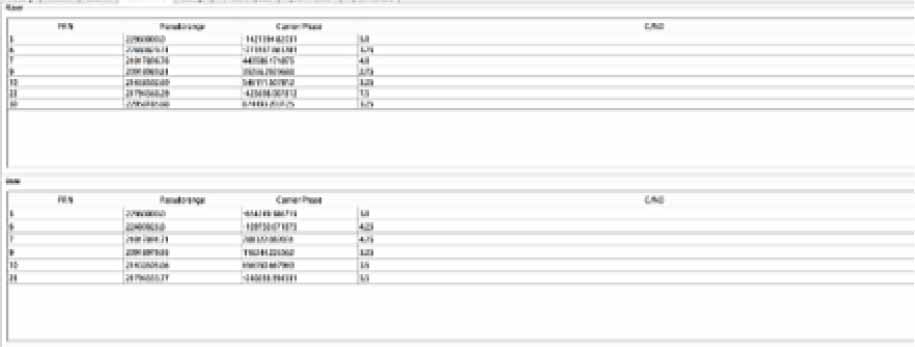
Figure 39.
Observation Screen
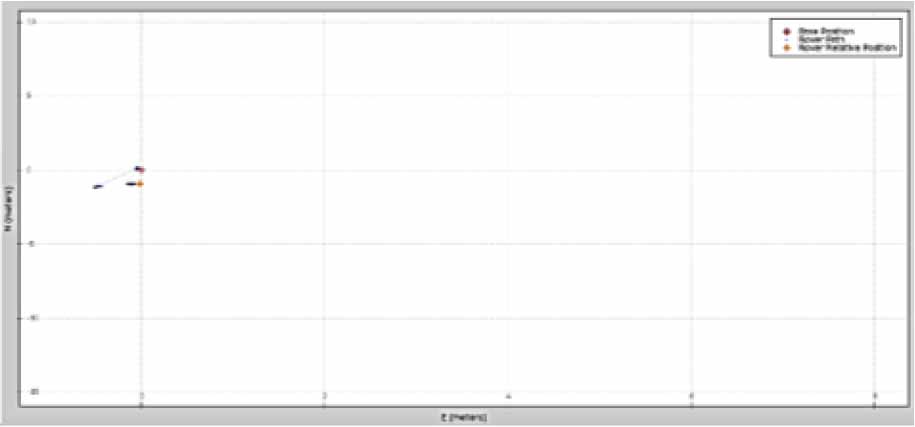
Figure 40.
RTK GPS positioning results 1
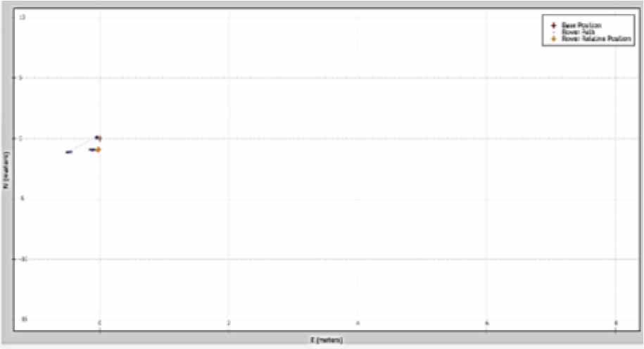
Figure 41.
RTK GPS positioning results 2
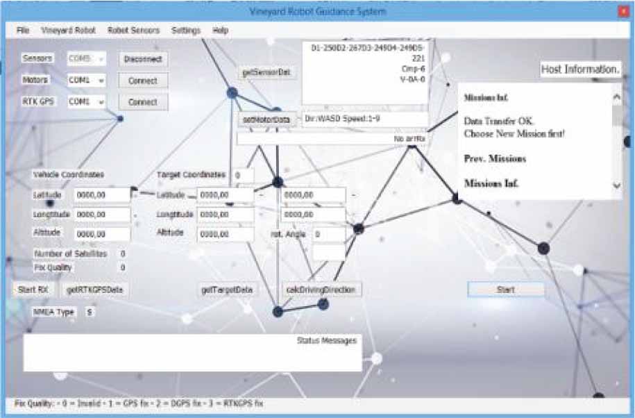
Figure 42.
Vineyard robot detection and control software
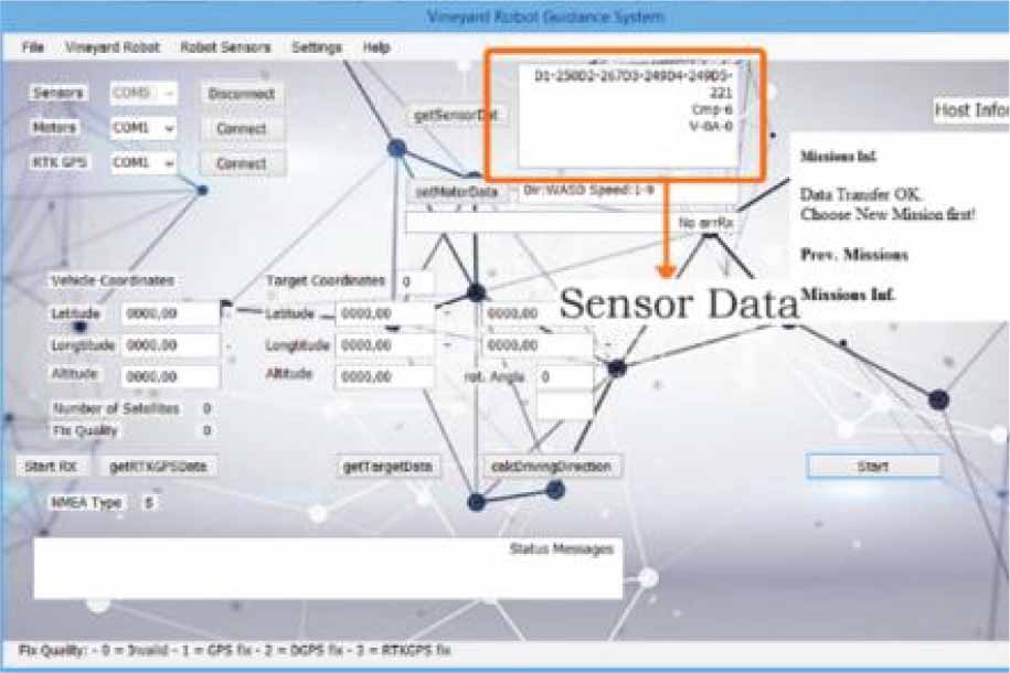
Figure 43.
Vineyard robot detection and control software - Sensor data
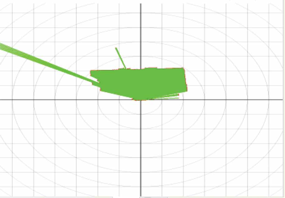
Figure 44.
Lidar measurement - Unobstructed conditions
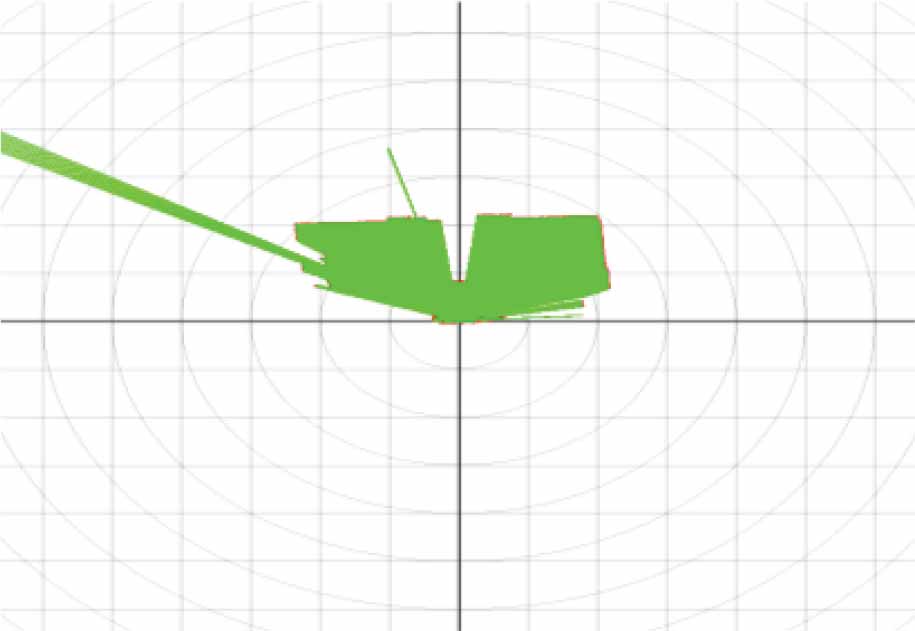
Figure 45.
Lidar measurement - Obstructed conditions
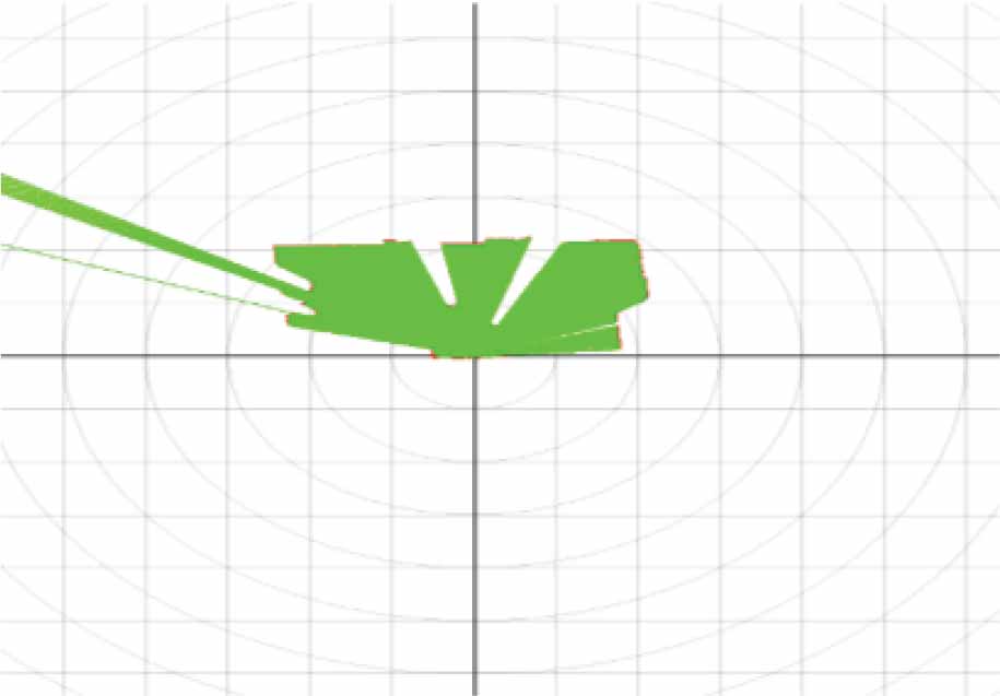
Figure 46.
Lidar measurement - Two obstacles present
Table 6.
Location Data Comparison Table
| Single Point Position (SPP) location data obtained with Piksi RTK GPS | Location data obtained using Google Maps | |
|---|---|---|
| Latitude (Decimal) | 37.8568583853 | 37.856858 |
| Longitude (Decimal) | 27.8582785723 | 27.858279 |
| Latitude (Degrees Minutes Seconds) | 37° 51’24.6902” N | 37° 51’ 24.7” N |
| Longitude (Degrees Minutes Seconds) | 27° 51’29.8029” E | 27° 51’ 29.8” E |
| Distance between the two acquired points (Decimal) | 0,00000039 | -0,00000043 |
| Distance between the two acquired points (Degrees Minutes Seconds) | 0° 0’0.0014” N | 0° 0’ 0.0015” W |
| Distance between the two acquired points (Meters) | 0.06455 m | |
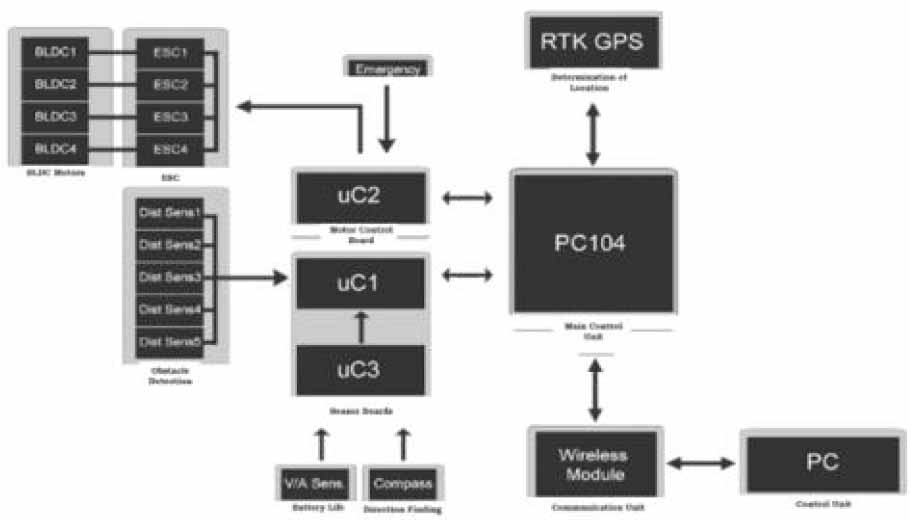
Figure 47.
Robot Control Architecture
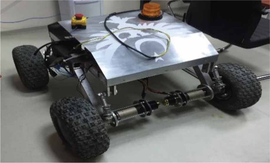
Figure 48.
Wheel-Based Agricultural Robot
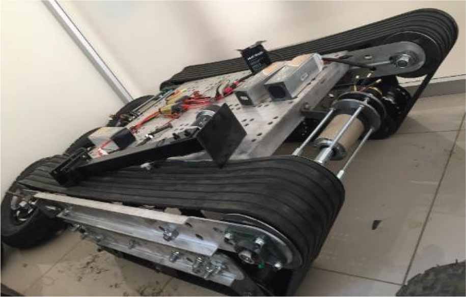
Figure 49.
Tracked Agricultural Robot