
Table 1.
Summary of the two 30-year simulations performed with NorESM.
Table 2.
Root-mean-squared errors of the PM2.5 downscaling relative to the pre-2005 AirBase measurements for the 2-level and 4-level approaches. The list of cities included in the different regions is provided in Figs. S1 and S2.
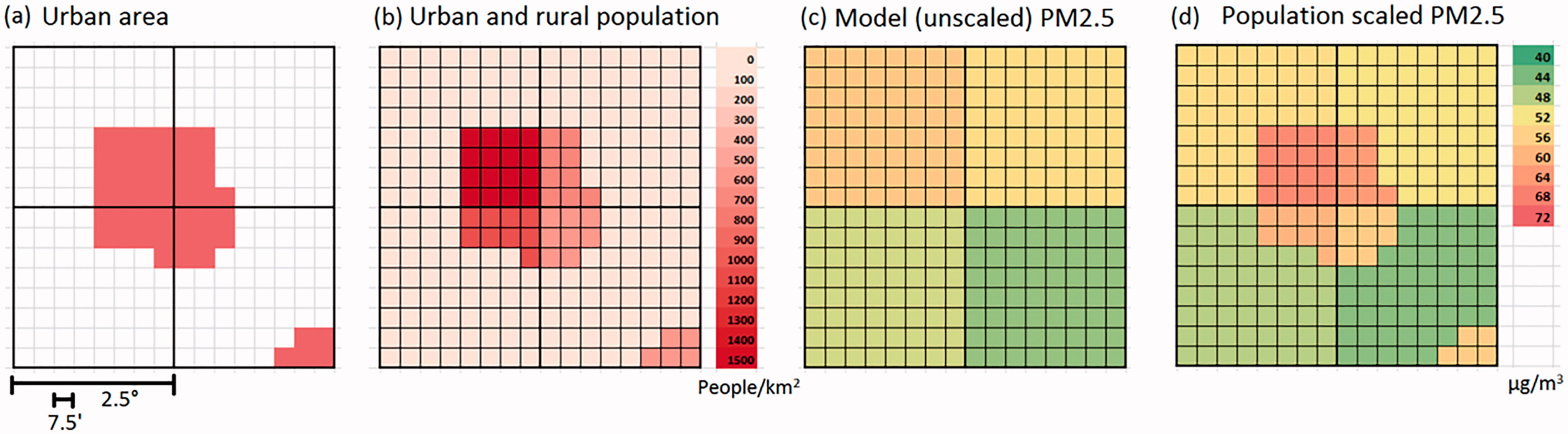
Fig. 1.
Schematic example of population scaling for four model grid cells. a) Fraction of urban area in model grid cells, red = urban, white = rural. b) Population density in model grid cells. The fraction of ρpop > 600/km2 is the fraction of urban population. c) Model grid PM2.5. d) Result of population scaling on PM2.5 (image courtesy of Rita van Dingenen).
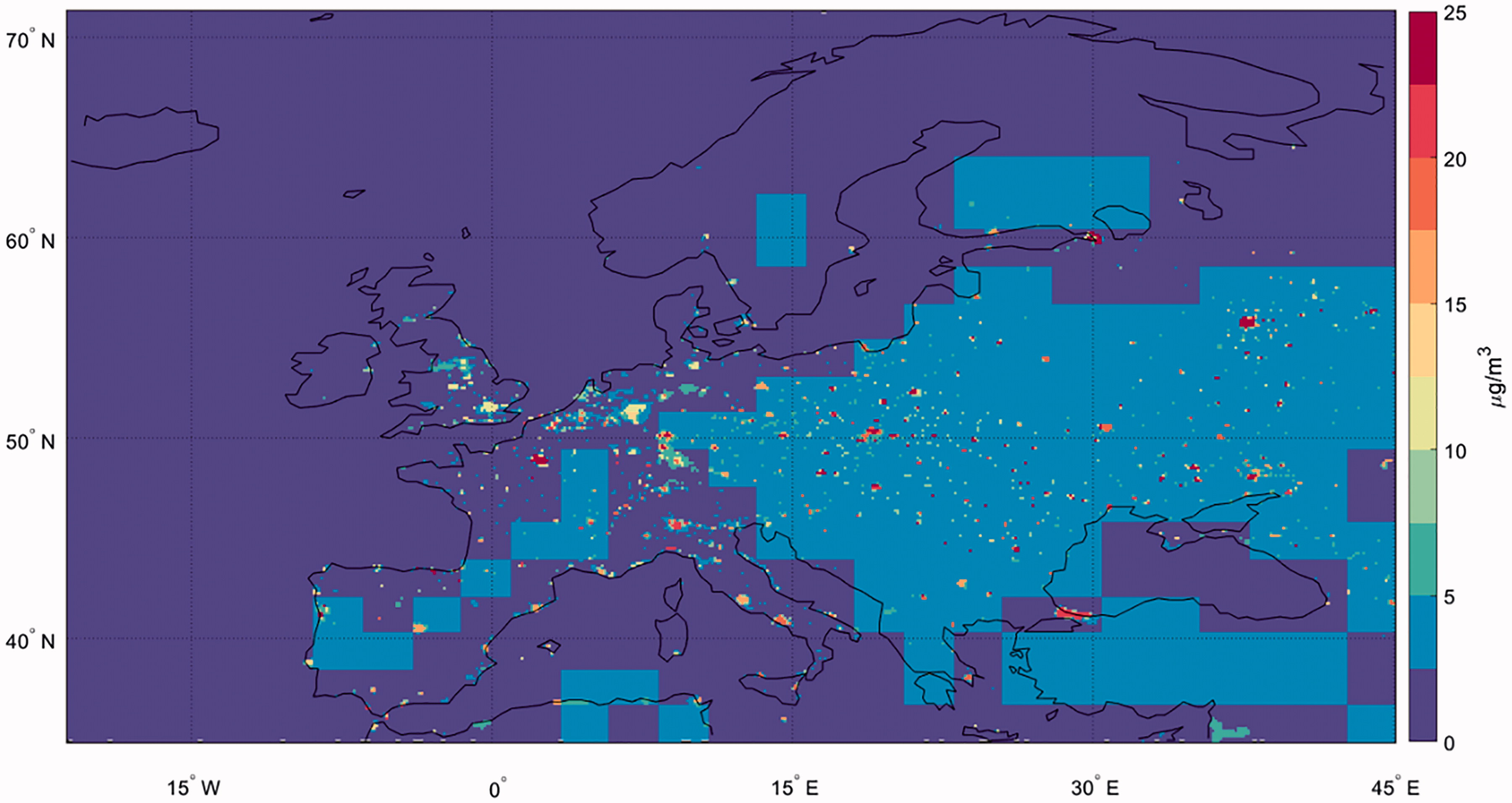
Fig. 2.
Annual average (2000–2005) population-weighted anthropogenic PM2.5, computed following the four-level downscaling approach described in Section 2.2.
Table 3.
Urbanization classes and empirically defined limits imposed on urban enhancement and rural reduction factors.
Table 4.
Summary of the different thresholds associated with PM2.5 guidelines.
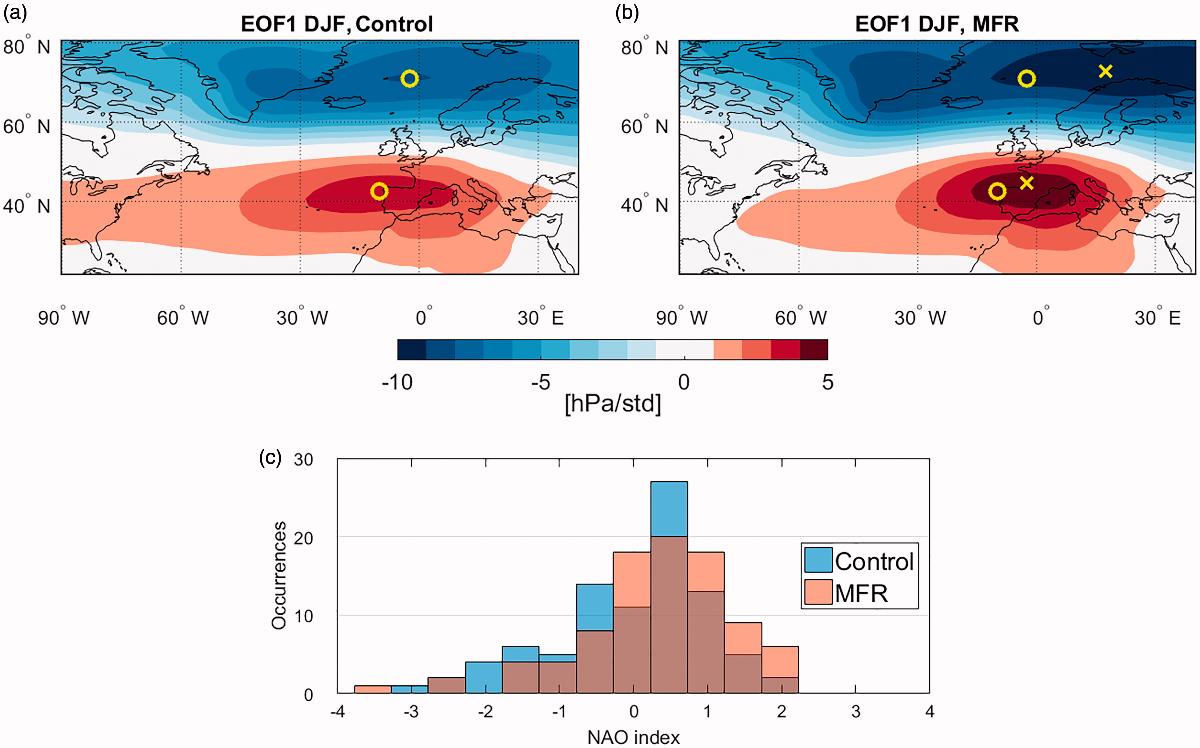
Fig. 3.
First EOF of sea level pressure for (a) the Control and (b) the MFR simulations, respectively. Circle (cross) markers indicate the Control (MFR) NACs. (c) Frequency distribution of the monthly NAOI for the Control (blue) and MFR (orange) simulations.
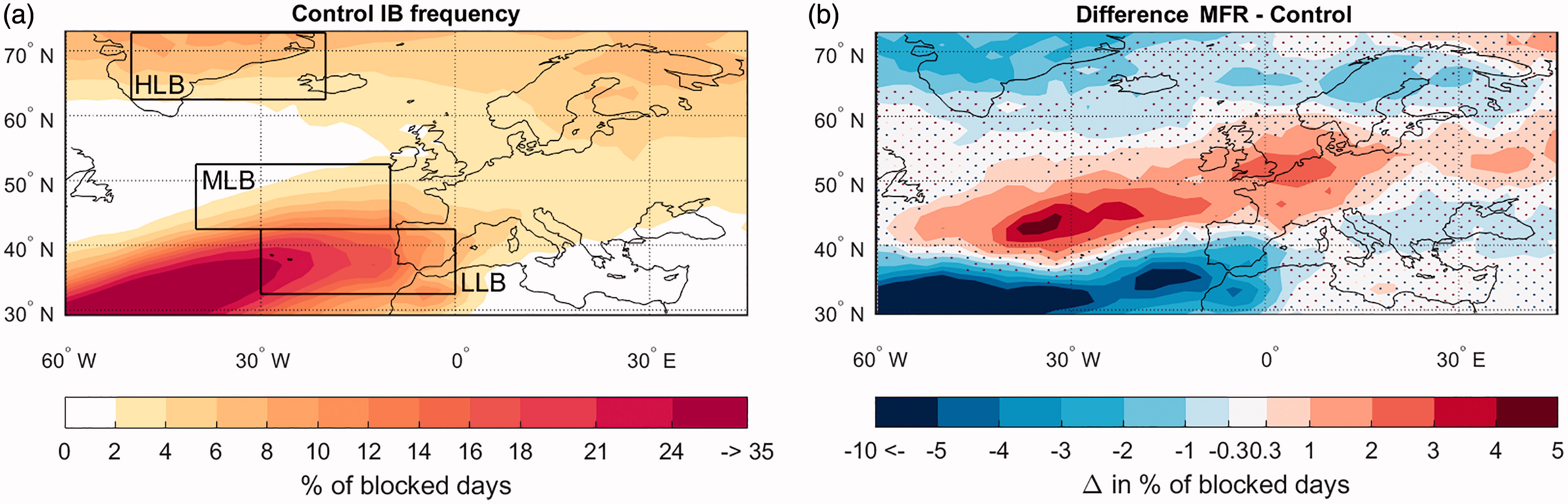
Fig. 4.
(a) Climatological DJF blocking frequency (% of blocked days) for the Control simulation. (b) changes in blocking frequency for the MFR scenario relative to the Control simulation. Stippling denotes areas where the difference is not significant at the 95% confidence level under a 2-sample t-test. The boxes in (a) mark the domains used to compute the low-, mid- and high-latitude blocking indices.
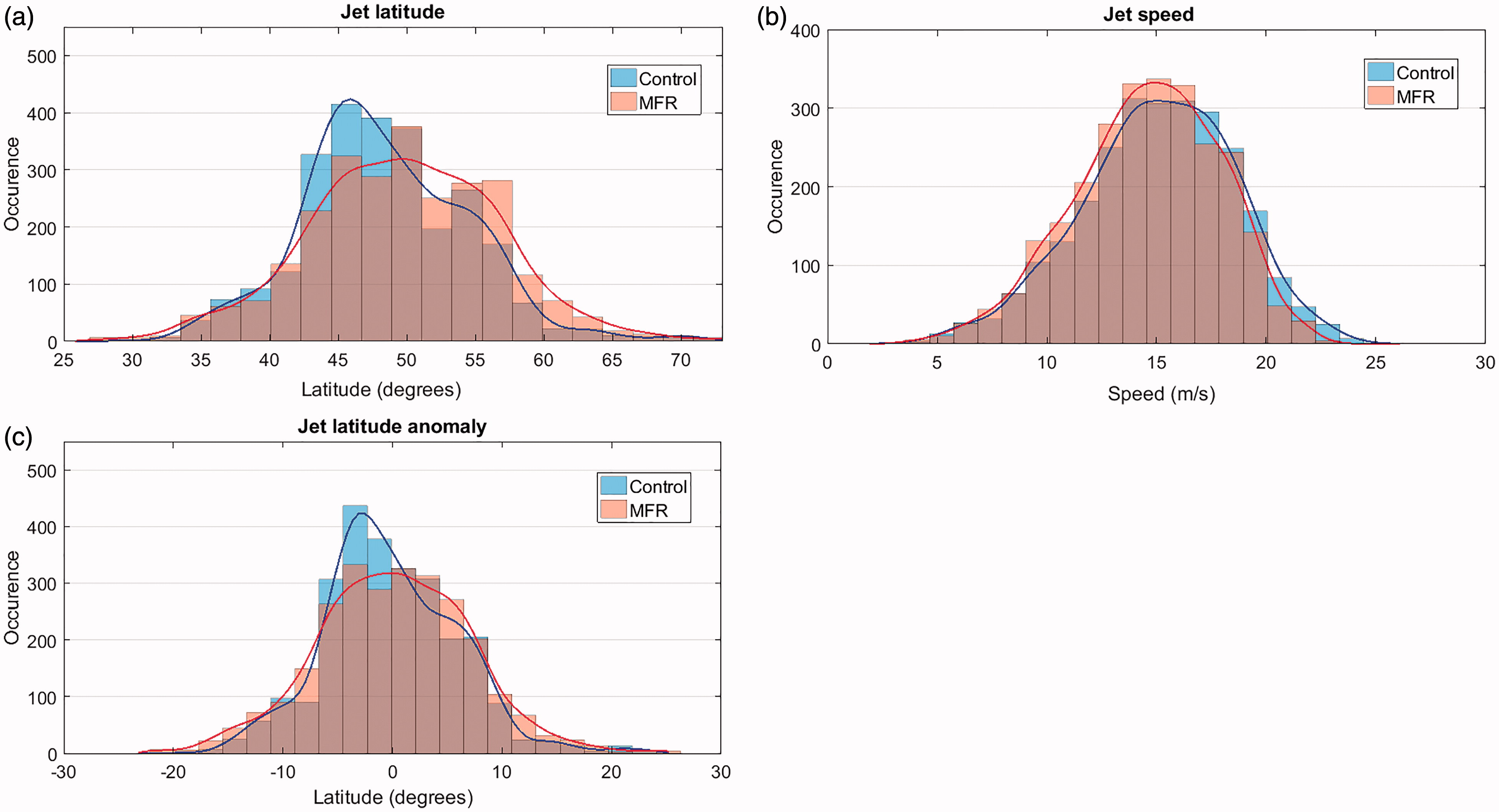
Fig. 5.
Frequency distributions of the daily DJF (a) jet latitude and (b) jet speed indices, for the Control (blue) and MFR (orange) simulations. Note that these are deviations from the seasonal cycle with the winter climatological means added back. (c) Displays the same distributions as (a) without the means added. The continuous curves are kernel estimations of the PDFs.
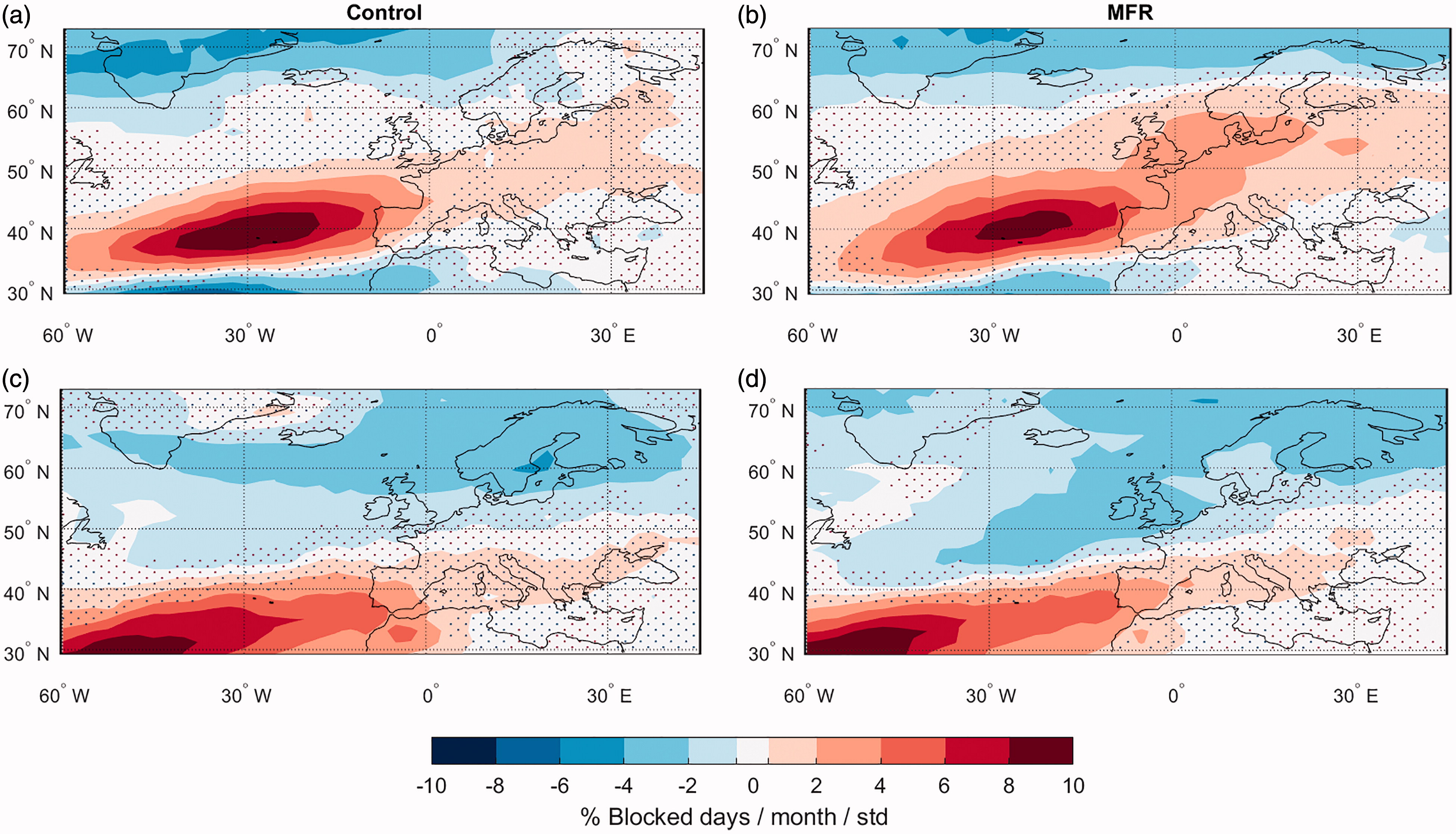
Fig. 6.
Regression patterns (% of blocked days/month/standard deviation) of blocking frequency on (a, b) jet latitude and (c, d) jet speed time series for the Control (a, c) and MFR (b, d) simulations during DJF. Stippling denotes areas where the regression is not statistically significant at the 95% confidence level, based on the standard error of the regression.
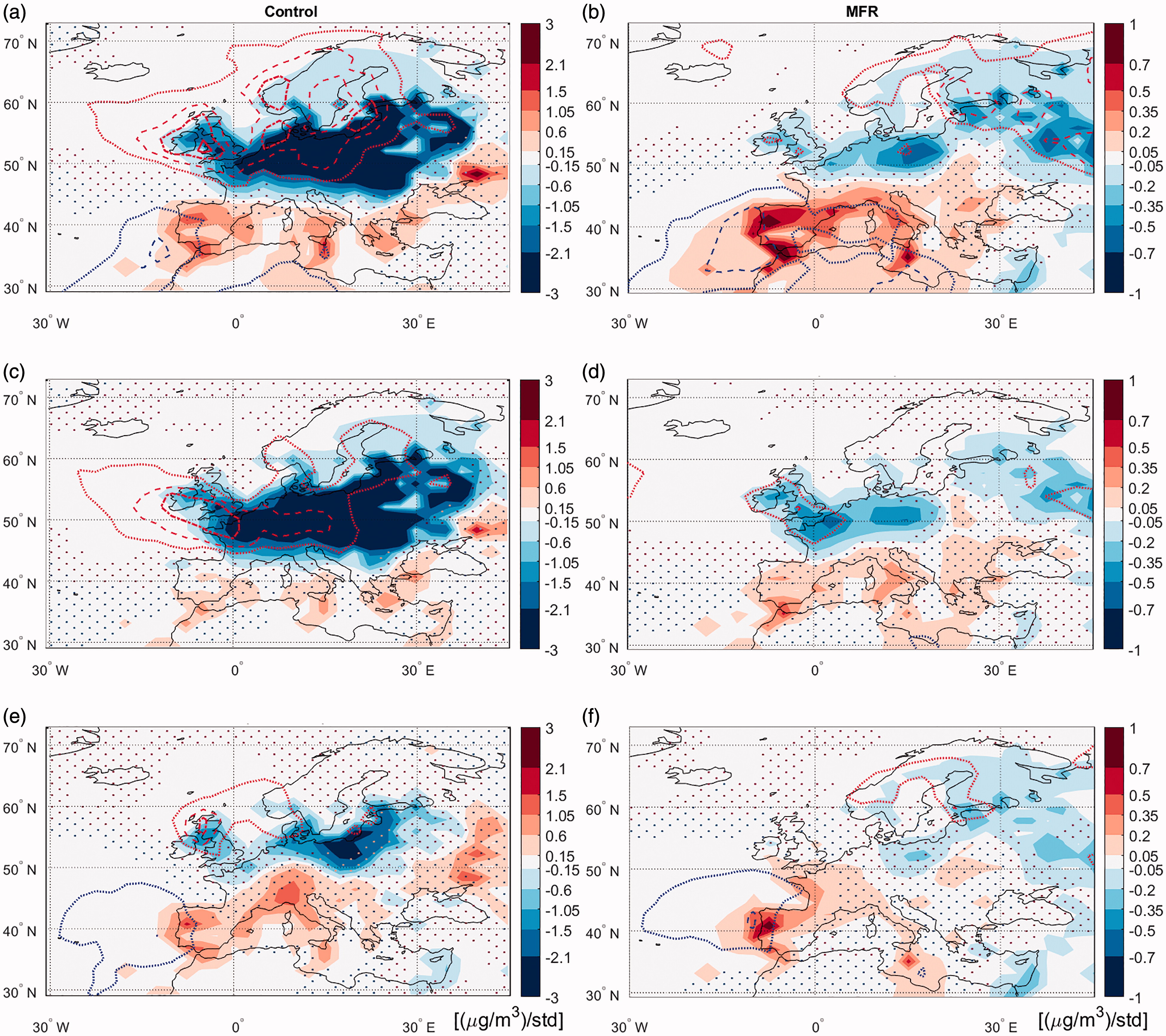
Fig. 7.
Regression patterns (µg/m3/standard deviation) of population-scaled urban anthropogenic PM2.5 anomalies on (a, b) the NAOI, (c, d) jet speed and (e, f) jet latitude indices, for the (a, c, e) Control and (b, d, f) MFR simulations during DJF. Line contours display positive (blue) and negative (red) departures from the DJF climatological mean, with contour intervals of 5%, starting from 10%. For enhanced visibility, contours change line style as follows: dotted, dashed, dash-dot, solid. Stippling denotes areas where the regression is not significant at the 95% confidence level, based on the standard error of the regression. Note that the colour scale ranges in the left and right-hand columns differ.
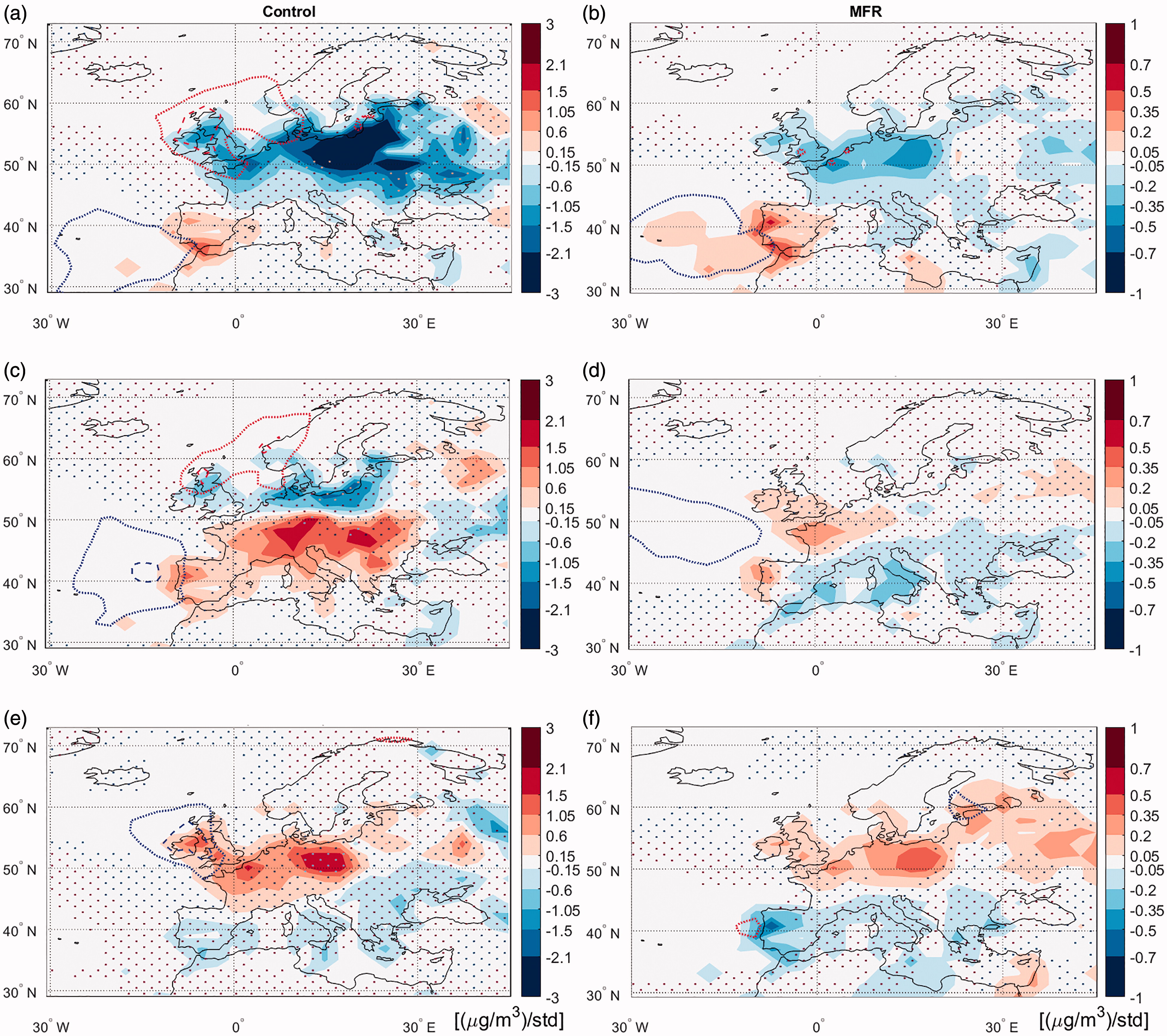
Fig. 8.
Regression patterns (µg/m3/standard deviation) of population-scaled urban anthropogenic PM2.5 anomalies on (a, b) LLB, (c, d) MLB and (e, f) HLB indices, for the (a, c, e) Control and (b, d, f) MFR simulations during DJF. Note that the colour scale ranges in the left and right-hand columns differ. All markings and colours are as in Fig. 7.
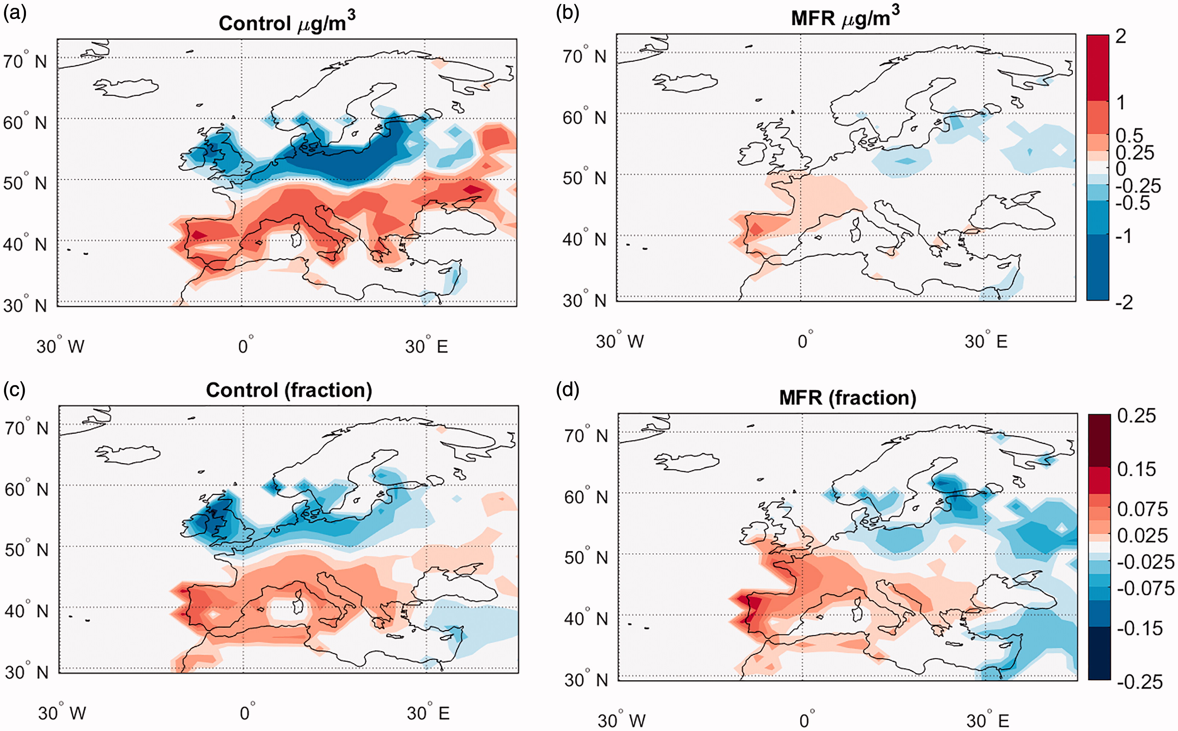
Fig. 9.
Climate penalty in PM2.5 concentrations for (a, c) the control and (b, d) the MFR simulations during DJF. This is expressed in terms of (a, b) absolute concentration values and (c, d) fractional changes relative to the DJF climatology.
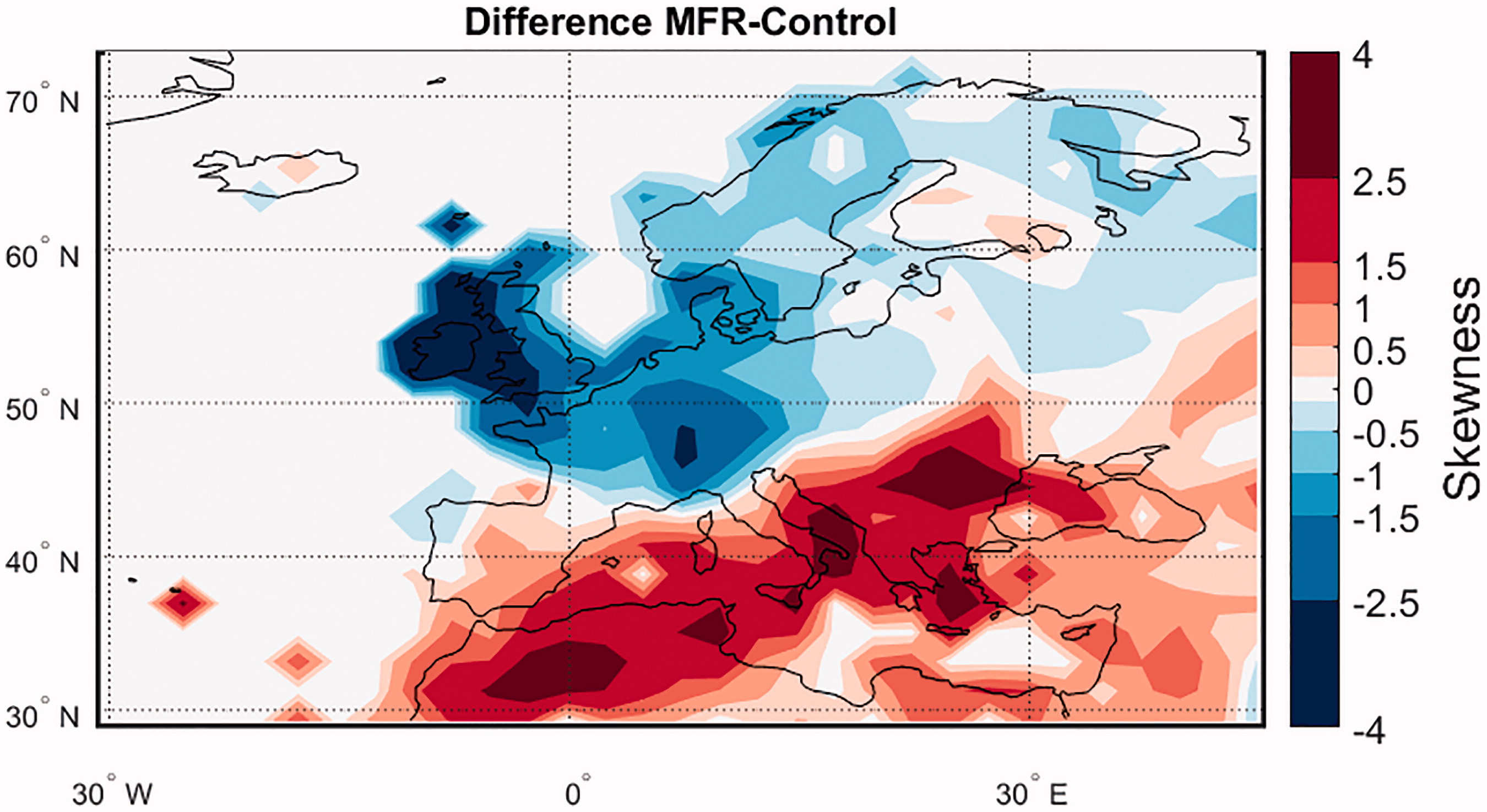
Fig. 10.
Difference in the skewness of the population-scaled urban anthropogenic PM2.5 between the Control and MFR simulations during DJF.
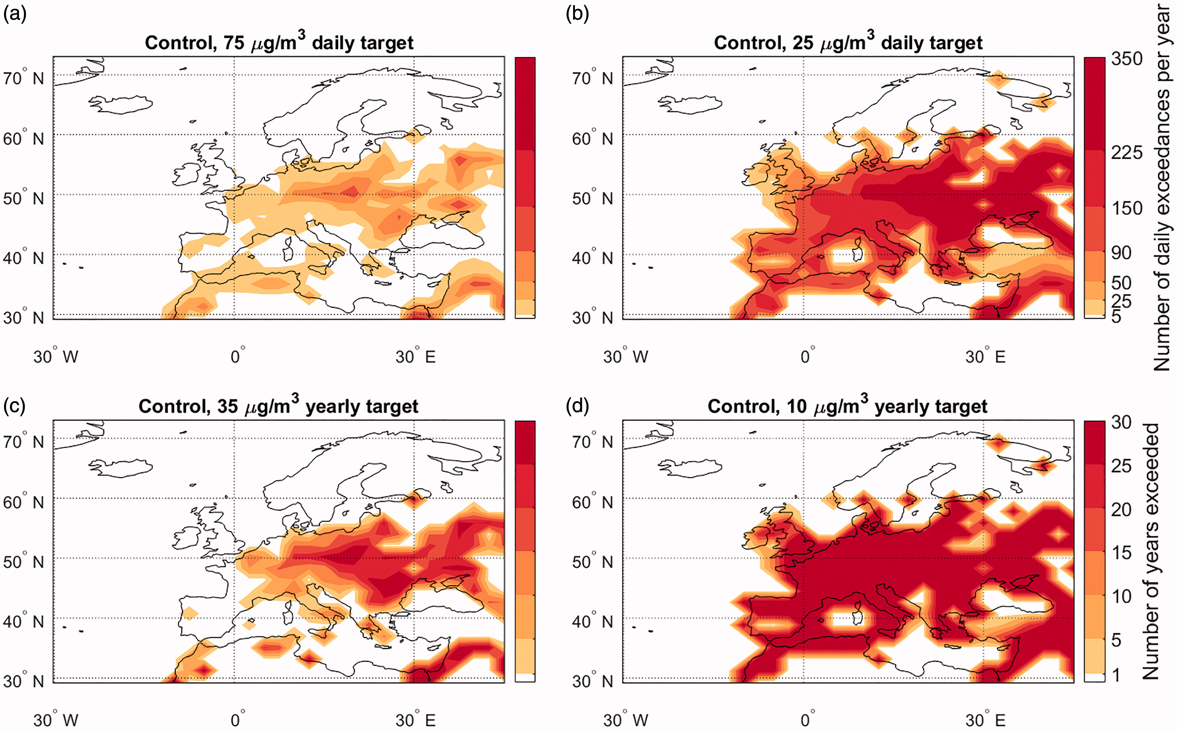
Fig. 11.
Exceedances of (a, c) the IT-1 and (b, d) the AQG PM2.5 aerosol limits in the control simulation. Results are expressed in terms of (a, b) the average number of days per year in which the daily targets were exceeded and (c, d) the number of years in which the yearly average targets were exceeded.
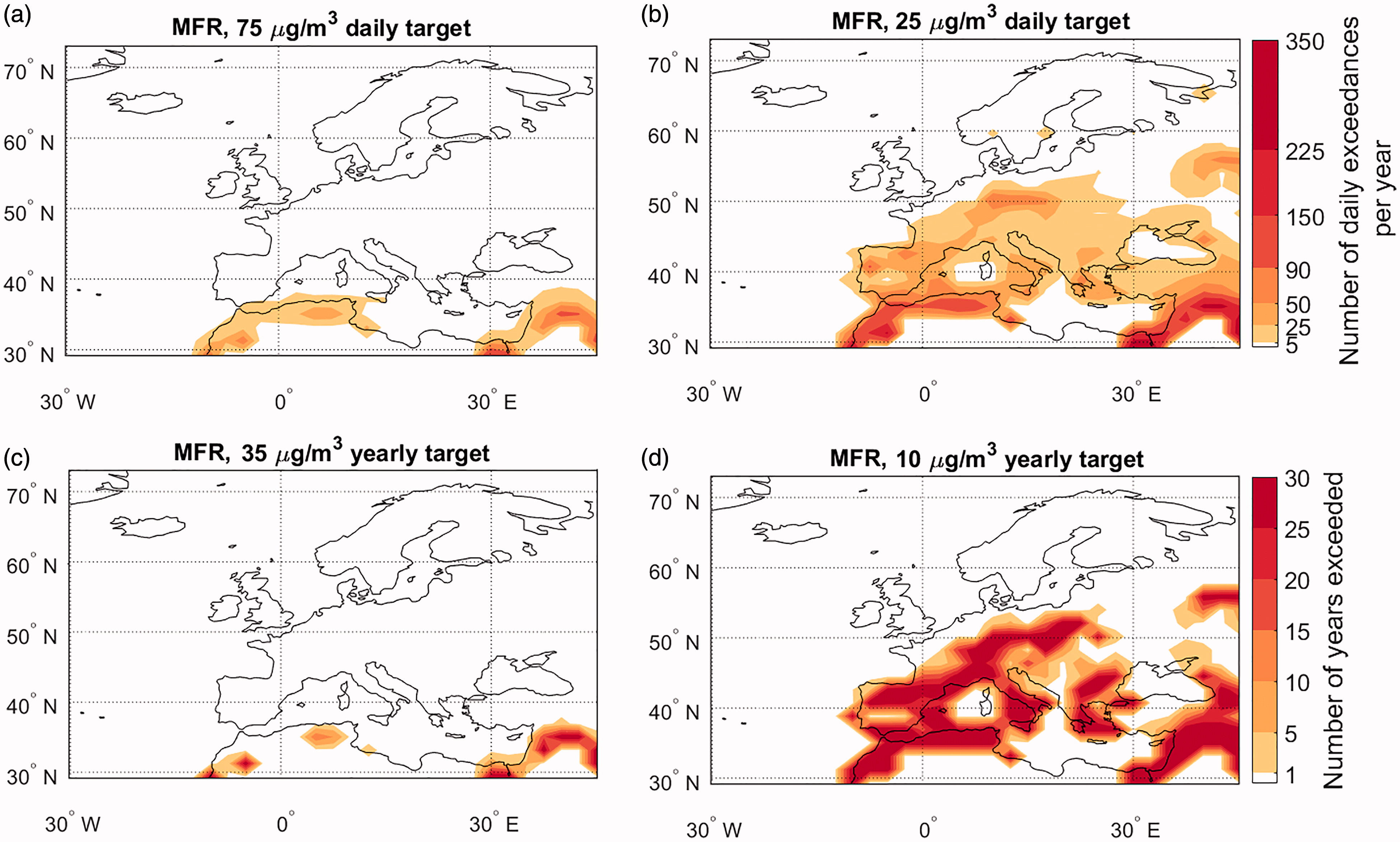
Fig. 12.
Exceedances of (a, c) the IT-1 and (b, d) the AQG PM2.5 aerosol limits in the MFR simulation. Results are expressed in terms of (a, b) the average number of days per year in which the daily targets were exceeded and (c, d) the number of years in which the yearly average targets were exceeded.