
Introduction
1.
High concentrations of airborne particulate matter (PM – a term referring to both solid and liquid particles) are associated with a wide range of acute and chronic health impacts, ranging from minor physiological issues to premature death from respiratory and cardiovascular diseases (e.g. Nel, 2005; Pöschl, 2005; Pope and Dockery, 2006; Araujo and Nel, 2009; Sapkota et al., 2012; West et al., 2016). Globally, over 2.5 million premature deaths per year are attributed to outdoor air pollution (WHO, 2014). Additional adverse impacts of PM (precursor) emissions comprise acid precipitation, effects on vegetation and reduced visibility (e.g. Grantz et al., 2003; Sun et al., 2006). Urban environments are particularly affected by many of these problems.
As a result of these detrimental effects, a number of governments and international organizations have introduced mandatory or recommended air quality limits for PM. In this paper we will focus on PM with an aerodynamic diameter below 2.5 μm (PM2.5). PM2.5 is considered more dangerous for health than coarser particles, since the smaller size allows it to penetrate further into the lungs heightening the risk of cardio-pulmonary diseases (WHO, 2005a; Boldo et al., 2006). The EU has set a target value of 25 μg/m3 for PM2.5 annual concentrations, (EEA, 2016), while the World Health Organization (WHO) has recommended a stricter annual threshold of 10 μg/m3 (Air Quality Guideline – AQG; WHO, 2005a). During 2012–2014, 8–12% of the urban population of the 28 European Union member countries was exposed to PM2.5 levels exceeding the current regulations. However, during the same period 85–91% has experienced levels above the more stringent AQG threshold. In 2013 alone, an estimated 4,668,000 years of life were lost in these countries as a result of air pollution (EEA, 2016).
European emissions of primary PM and precursor gases show a decreasing trend (e.g. Tørseth et al., 2012; Maas and Grennfelt, 2016), also thanks to continued regulatory efforts. However, the actual PM concentrations can be heavily affected by both local meteorological conditions (e.g. Barmpadimos et al., 2011; Czernecki et al., 2017) and large-scale anomalies in the atmospheric circulation (e.g. Eckhardt et al., 2003; Christoudias et al., 2012; Barnes and Fiore, 2013; Pausata et al., 2013; 2015). In particular, the North Atlantic Oscillation (NAO) has been identified as an important control of regional-scale pollutant concentration variability across Europe (e.g., Pausata et al., 2012, 2013). The NAO is the leading mode of atmospheric variability in the North Atlantic region, especially during winter, and is typically quantified in terms of the sea-level pressure difference between the Icelandic low and the Azores high (Walker and Bliss, 1932; Hurrell et al., 2003). A positive NAO is characterized by an enhanced westerly flow, leading to wetter and milder conditions over the northern part of Europe and drier conditions over the Mediterranean area. Pausata et al. (2013) found that the NAO can account for a large fraction of the interannual variability in PM2.5 concentrations in the present climate, with a positive NAO leading to increased concentration anomalies in the Mediterranean region and negative anomalies in central-northern Europe. This control can be primarily ascribed to the direct meteorological impact of the NAO on PM concentrations (e.g. changes in wet and dry deposition through changes in rainfall and wind speed), but may also be mediated by the effect of the different prevailing weather conditions on anthropogenic PM emissions (e.g. altered domestic heating demand and choice of modes of transport).
Conversely, the aerosols themselves can have short-term impacts on climate through a range of direct and indirect effects (Shindell et al., 2012; Acosta Navarro et al., 2017). Global climate models must take into account both greenhouse gases (GHGs) and aerosols to capture the temperature trend of the last century (e.g. Nazarenko and Menon, 2005; Gleckler et al., 2008; IPCC 2013). Aerosol concentrations will thus play an important role in determining the future climate but may in turn be affected by the climate itself, driving a complex set of interactions and feedback mechanisms.
Long-term global scenarios for air pollutant emissions have been used in climate models to simulate future climate change. These scenarios project plausible future emissions based on socioeconomic, environmental and technological trends (Moss et al., 2010). A number of modelling studies suggest a future positive shift in the NAO as part of anthropogenic climate change (e.g. Hu and Wu, 2004; Kuzmina et al., 2005; Karpechko, 2010; Gillet and Fyfe, 2013). The changing weather patterns associated with a more positive NAO will likely affect PM concentrations across Europe, with potentially major impacts on public health (Pausata et al., 2013). At the same time, the ongoing downward trend in European anthropogenic aerosol emissions may be one of the drivers contributing to the modelled NAO shift. Pausata et al. (2015) showed that under a scenario of maximum feasible aerosol emission abatement the aerosol decrease alone may lead by 2030 to a positive shift in the NAO mean state comparable to that driven by increased greenhouse gas concentrations. Long-term pollutant reduction goals should therefore account for the effects of future circulation changes (Pausata et al., 2015).
The spatial resolution of climate models is typically too coarse to study local PM variability. Deterministic and statistical downscaling models have therefore been widely used to extract high-resolution pollutant concentrations from model simulations of historical and future climates. Deterministic models, such as chemistry transport models and high-resolution regional air quality models, compute pollutant concentrations as explicit functions of meteorological parameters, chemical transformation processes and source characteristics, and can consequently be computationally expensive (e.g. Liora et al., 2016; Syrakov et al., 2016; Hong et al., 2017). Statistical models are instead based on the relationship between observed small-scale variables (predictands) and large-scale fields from a numerical model (predictors), and are generally computationally inexpensive (Wilby et al., 2004). These modelling and downscaling efforts are complemented and supported by high-resolution pollutant inventories (e.g. Kuenen et al., 2014; Dernier et al., 2015). For an overview of air quality modelling approaches, we refer the reader to Rouil and Bessagnet (2013).
In this study, we consider a historical control scenario and a future scenario of maximum feasible aerosol reduction (MFR), consistent with the implementation of the most advanced emission reduction technologies presently available. We combine an analysis of daily urban-scaled PM2.5 concentrations in both scenarios with a detailed study of the projected atmospheric circulation changes in the Euro-Atlantic sector. We focus on the boreal winter season (December–February) which typically displays the most severe PM pollution episodes (Dos Santos et al., 2015). We aim to improve our understanding of the interplay between the atmospheric circulation and aerosol concentrations, which is essential in supporting the development and implementation of future aerosol regulations. Specific objectives of our study are to:
Provide a full analysis of the atmospheric circulation changes under an MFR scenario (see Section 2.1), including changes in the location and speed of the jet stream and in blocking events. The majority of past studies on the topic have focussed on changes in the NAO; however, the NAO alone provides an incomplete description of the atmospheric variability in the Euro-Atlantic sector, and only explains part of the jet stream’s deviations from climatology (Woollings et al., 2010).
Implement and validate a novel population-based downscaling method for estimation of urban PM2.5 concentrations in a global modelling context. While high-resolution regional models (e.g. Liora et al., 2016; Syrakov et al., 2016; Galmarini et al., 2017; Hong et al., 2017) and more complex downscaling methodologies (e.g. Milionis and Davies, 1994; Kumar and Goyal, 2016) than the one used here might, in theory, yield better results (Thunis et al., 2016), computational constraints make their application to climate timescales and continent-wide studies challenging. This study satisfies the need to have an improved first-order downscaling scheme that addresses population-weighted impacts.
Verify the impact of the atmospheric circulation changes on the downscaled urban PM2.5 concentrations and evaluate implications for air quality regulations. The jet stream’s variability is linked to surface wind and precipitation variability over Europe (e.g. Hanley and Caballero, 2012; Messori and Caballero, 2015; Messori et al., 2016) and can affect PM2.5 concentrations through changes in transport and wet and dry deposition. It is therefore important to include other atmospheric circulation indices besides the NAO to provide a more complete picture of the aerosol-circulation interactions over Europe.
Verify whether the Norwegian Climate Centre’s Earth System Model (NorESM) used here reproduces changes in atmospheric circulation and impacts on air pollution similar to those seen in previous studies which used an MFR scenario – such as Pausata et al. (2015). The latter study was performed using a general circulation aerosol model (ECHAM5-HAM) coupled to a mixed layer ocean, therefore neglecting potential feedbacks on the atmosphere due to anthropogenic-induced changes in ocean circulation. It is therefore important to validate these earlier findings.
A detailed description of the simulations and the analysis methods used is provided in Section 2. Section 3 describes the future atmospheric circulation changes and their impact on urban air quality across Europe. Finally, the implications of our analysis for future air quality regulations and the conclusions are presented in Section 4.
Data and methods
2.
Climate model description, simulation setup and additional data
2.1.
This study is based on two 30-year simulations performed with the Norwegian Earth System Model (NorESM1-M; Bentsen et al., 2013). The version of NorESM used in this study participated in the Coupled Model Intercomparison Project phase 5 (CMIP5, Taylor et al. (2012)). The atmospheric component, CAM4-Oslo, has a finite volume grid with a horizontal resolution of 1.9° latitude by 2.5° longitude, and 26 vertical levels. It includes an interactive aerosol module that provides a physical description of aerosol processes and their interactions with radiation and clouds (Kirkevag et al., 2013). The model represents black carbon (BC), organic matter (OM), sulphate (SO4), sea salt (SS), mineral dust (DU) and the precursor gases dimethyl sulphide (DMS) and sulphur dioxide (SO2). The OM/Organic Carbon (OC, the carbon fraction of OM) ratio used is 2.6 for biomass burning OC and 1.4 for the rest (e.g fossil fuel OC, secondary organic aerosols etc.). Dry aerosol particles are affected by ambient humidity in two ways. At sub-saturation (i.e. RH < 100%) aerosol particles take up water and grow in size depending on the particles’ hygroscopicity. At supersaturation (i.e. RH > 100%) aerosol particles can activate to form cloud droplets following Köhler theory. Therefore, the model takes into account the direct aerosol effect, cloud albedo and cloud lifetime effects on climate. Oxidant fields are prescribed following the approach of Kirkevag et al. (2013).
The two simulations performed are: 1) a historic (1976–2005) control simulation with prescribed historic aerosol emissions and GHG concentrations as used in the IPCC AR5 report (IPCC, 2013); 2) a future (2037–2066) simulation based on the MFR aerosol scenario (Cofala et al., 2007; Klimont et al., 2016) and Representative Concentration Pathway 4.5 (RCP4.5) GHG concentrations (Thomson et al. 2011; IPCC, 2013). Aerosol and aerosol precursor emissions follow Lamarque et al. (2010) between 1976 and 2000 and the IIASA ECLIPSE V4a MFR after 2005, with a linear interpolation between 2000 and 2005. The MFR scenario describes global aerosol emission levels up to 2030 in the case of a strong abatement of anthropogenic aerosol emissions by the implementation of the most advanced emission control technologies available today. Globally, this corresponds to an emissions decrease of 47% for BC, 60% for OC and 77% for SO2 emissions (the main anthropogenic precursor of SO4) by 2030 compared to 2000 levels. Natural and anthropogenic biomass burning emissions are kept constant at 2000 levels; similarly, changes in land use and emissions due to aviation and shipping are not taken into account. As a caveat, we note that the IMO (International Maritime Organization) agreements on shipping regulations may lead to significant emission changes over the oceans and coastal regions after 2020 (IMO, 2008). DU emissions are prescribed at present-day levels and SS emissions are dependent on sea surface temperature and 10-meter wind speed (Struthers et al., 2011). The simulation for the future climate uses constant 2030 MFR aerosol and precursor emissions over the entire 2037–2066 period. While it may be reasonable to expect that pollutant concentrations continue to decrease in the future, the enforcement success of future targets is difficult to predict. Furthermore, assumptions on air pollution control should be consistent with the concurrent challenges to climate change mitigation and adaptation (Rao et al., 2017). We therefore assume that PM emissions will level off at 2030 MFR values and will remain steady overall during the period analyzed. Due to the time-varying forcings, the PM data is detrended before analysis, except when computing regulatory threshold exceedances. A summary of the simulations is given in Table 1.
Table 1.
Summary of the two 30-year simulations performed with NorESM.
We further make use of the European Centre for Medium Range Weather Forecasts’ ERA-Interim reanalysis data (Dee et al., 2011), to evaluate the model’s performance in reproducing atmospheric blocking and the jet stream’s variability. We use data with a horizontal resolution of 1° × 1°.
PM downscaling
2.2.
The model’s horizontal resolution limits the ability to assess urban air pollution and regulation exceedances. To overcome this issue, the PM2.5 components with a predominantly anthropogenic emission signature (BC, OM, SO4) are downscaled to a resolution of 7.5′×7.5′ (∼15 km × 15 km) using population density. The latter is based on the high resolution SEDAC database (SEDAC, 2005), mapped to a 7.5′ × 7.5′ horizontal grid. The highest population densities are systematically associated with urban centres and high anthropogenic aerosol emissions. The anthropogenic aerosol concentrations tend to show a similar pattern to the emissions, and dilute rapidly as the distance from the sources increases. As a caveat of our methodology, we note that the same population density is used for both the historic and the future simulations. This is further discussed in Text S1 in the Supplementary Material.
In the control simulation, the individual BC, OM and SO4 components contribute to ∼10%, 50%, and 25% of the total PM2.5 over the European continent, respectively (not shown). The BC and OM concentrations show a very local signature over urbanized regions, and are therefore fully included in the downscaling. SO4 originates from a mix of both anthropogenic and natural emission sources and mixing with natural aerosols, and typically has a regional-scale signature. However, all SO4 is downscaled in order to account for the absence of NOx from anthropogenic sources in CAM4-Oslo’s aerosol module. This approximation was previously implemented in Pausata et al. (2013). While there are certainly differences in both the origin and distribution of sulphates and nitrates, the two share broadly similar regional patterns (urban/semi-urban characteristics), justifying such an approach. Aerosol components of predominantly natural origin (SS, DU) are not modified.
Previous studies addressing global or continent-wide urban aerosol concentrations under different scenarios have typically applied a 2-level aerosol downscaling, subdividing model grid boxes into urban and rural areas (e.g. Leitãoa et al., 2013; Pausata et al., 2013). Here we instead consider four distinct urbanisation levels: urban centres (ρpop > 1000 people/km2), urban background areas (1000 ≥ ρpop > 600 people/km2), rural background areas (600 ≥ ρpop > 300 people/km2) and natural background areas (ρpop ≤ 300 people/km2). Throughout this study, urban centre values are referred to as urban PM concentrations. The sum of BC, OM and SO4 aerosol concentrations for each grid box is weighted according to this subdivision, resulting in four distinct values per grid box. All grid box means are preserved in this process. This effectively implements a redistribution of the coarse model grid anthropogenic PM2.5 according to population density. Unlike in the 2-level downscaling, the separation into four sublevels creates a PM concentration gradient that distinguishes between large cities, small cities and rural areas. Rural concentrations are more realistic and an additional PM enhancement is obtained for the largest cities. This generally results in an improved agreement with in-situ urban PM2.5 measurements (AirBase data, EEA, 2013; Table 2). In regions characterised by small or medium-sized urban centres surrounded by predominantly rural areas, such as often found in Eastern Europe, the performance of the two methods is comparable. A more detailed validation of the downscaling is presented in Text S2 in the Supplementary Material.
Table 2.
Root-mean-squared errors of the PM2.5 downscaling relative to the pre-2005 AirBase measurements for the 2-level and 4-level approaches. The list of cities included in the different regions is provided in Figs. S1 and S2.
For each model grid cell, an urban area fraction f Α, urb , and an urban population fraction f pop,urb are computed according to:
where ΣAurb (i, j) is the urban area within the total area, ΣA(i, j), of each model grid cell, Σρpop ,urb(i,j) = ρpop · Α urb is the urban fraction of the total population Σρpop (i,j), and i and j are the latitude and longitude indices of the 7.5 ′× 7.5′ population density grid. Iterating this process provides the equivalent fractions for the urban centre (urb_centre) and urban background (urb_back) regions:Exactly the same methodology is then applied to determine the rural (rur_back) and natural (rur_nat) background fractions. The enhancement and reduction factors for urban and rural areas, respectively, are then defined as:
Equations (5) and (6) are then used to define urban and rural aerosol backgrounds:
Two further weighting factors are then defined for the two classes of urban environments as:
The two corresponding rural scaling factors, PFUrur and PFRrur , are defined in an analogous fashion. The downscaled anthropogenic PM2.5 is finally obtained as:
Figure 1 provides a simplified scheme of the downscaling procedure for the 2-level (urban and rural) scaling. Because the enhancement factors are inversely proportional to the area fractions, concentrations in isolated cities within sparsely populated regions or densely populated regions with small urban centres are unrealistically enhanced, while the inverse happens in the corresponding rural areas. Therefore, we place limits on the values of the enhancement factors. The different thresholds are listed in Table 3. We note that this additional step is not specific to our 4-level downscaling, and is necessary also in the 2-level case. The final downscaled, population-weighted PM2.5 concentrations over Europe, as defined in Equation 11, are shown in Fig. 2. A comparison with the AirBase in-situ urban PM2.5 measurements over the period 2000–2005 (EEA, 2013) shows that the ranges of the downscaled model values and observed concentrations overlap for all cities in the dataset (see Supplementary Material).
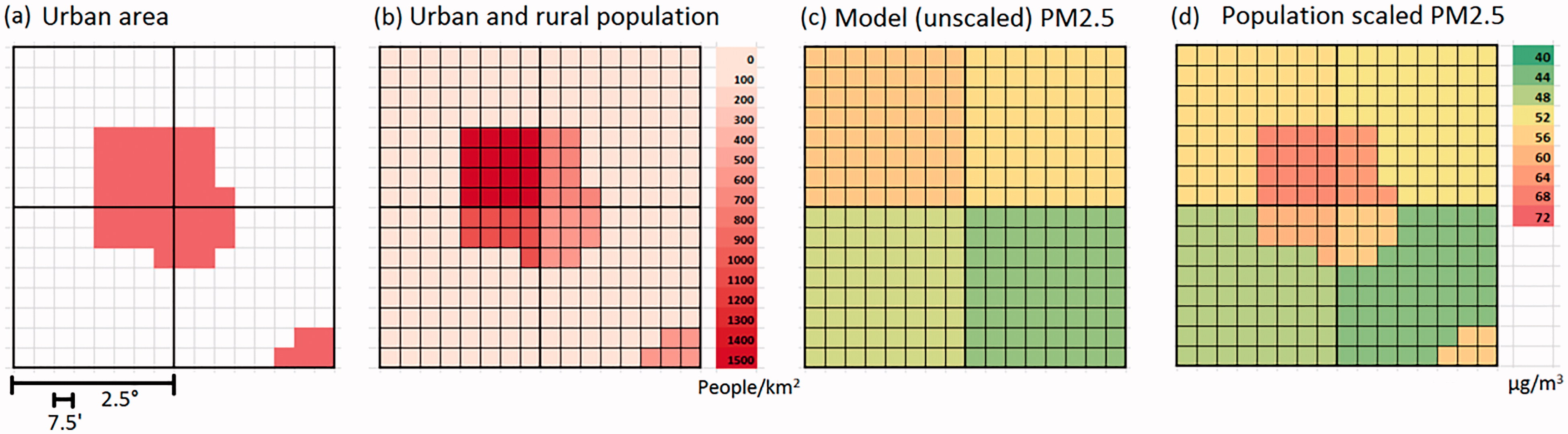
Fig. 1.
Schematic example of population scaling for four model grid cells. a) Fraction of urban area in model grid cells, red = urban, white = rural. b) Population density in model grid cells. The fraction of ρpop > 600/km2 is the fraction of urban population. c) Model grid PM2.5. d) Result of population scaling on PM2.5 (image courtesy of Rita van Dingenen).
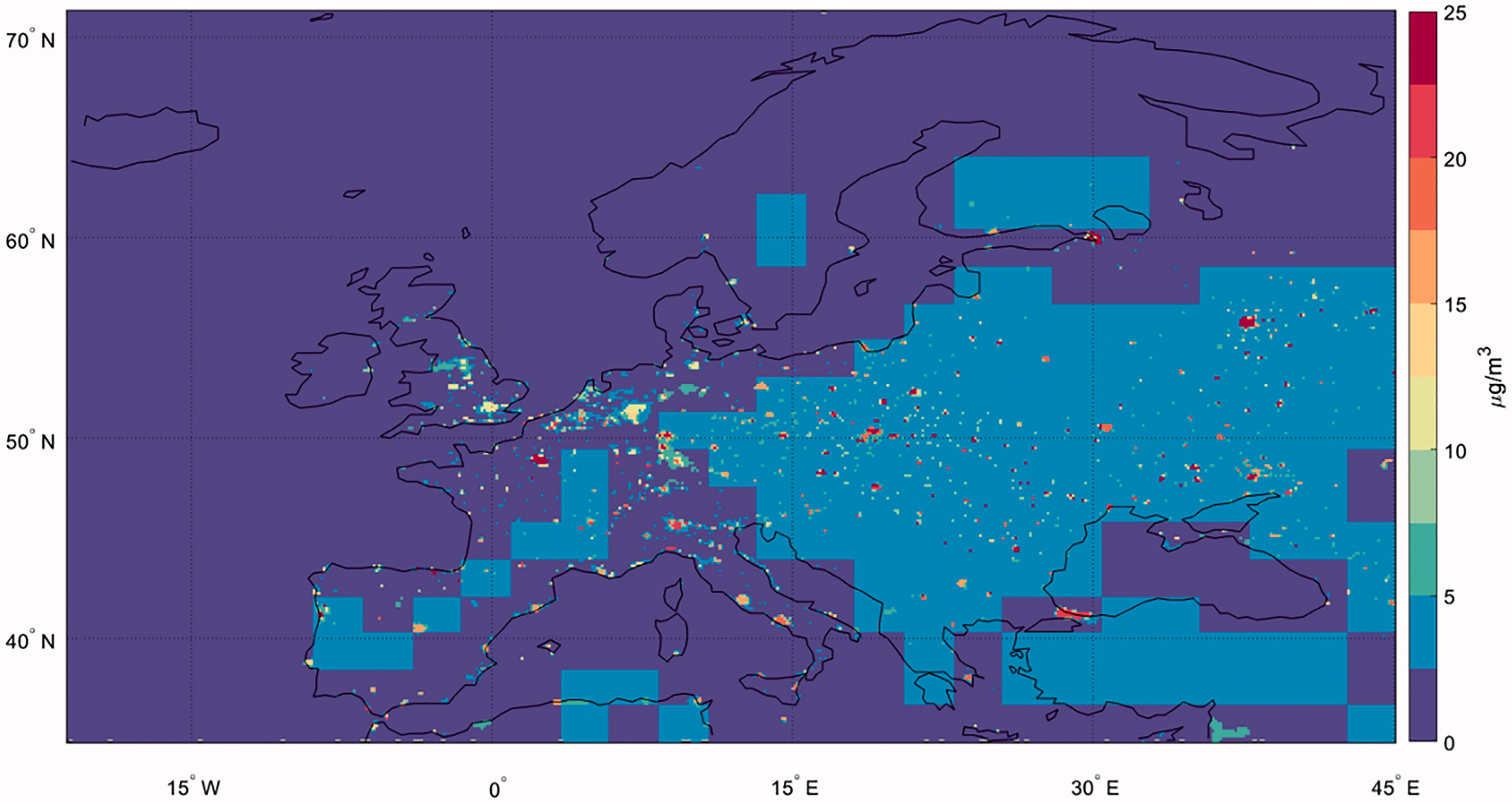
Fig. 2.
Annual average (2000–2005) population-weighted anthropogenic PM2.5, computed following the four-level downscaling approach described in Section 2.2.
Table 3.
Urbanization classes and empirically defined limits imposed on urban enhancement and rural reduction factors.
PM regulations
2.3.
The EU’s Air Quality Directive annual target of 25 μg/m3 for PM2.5 was introduced on the 1st January 2015. Before this date, no specific PM2.5 concentration limits were set by EU legislation. EU daily PM2.5 limits are yet to be enforced. The WHO has defined a set of Air Quality Guidelines (AQG), namely limits based on the lowest PM2.5 concentration levels at which adverse health effects have been shown to occur with more than 95% confidence in response to long-term exposure (WHO, 2005a). These limits should therefore be seen as the long term target for all air quality policies, and are considered by the WHO to be ‘achievable in large urban areas in highly developed countries’ (WHO, 2005b; p. 9). The AQG limits are 10 μg/m3 on an annual basis and 25 μg/m3 on a daily basis. The annual limit is less than half of the EU’s Air Quality Directive target.
The WHO has further defined a series of interim targets, which are intended to provide a means for policy makers to gauge progress in reducing the population’s exposure to PM. The IT-1 (Interim Target 1) limits correspond to PM2.5 concentrations that have been shown to lead to significant mortality in the developed world (WHO, 2005a). These should therefore be viewed as a target that needs to be attained with some urgency. The IT-1 limits are 35 μg/m3 on an annual basis and 75 μg/m3 on a daily basis. The annual limit is therefore higher than the EU’s Air Quality Directive target. Table 4 provides a summary of the different WHO limits discussed here.
Atmospheric dynamics and climate indices
2.4.
In order to investigate wintertime changes in the large-scale atmospheric variability, we analyse the jet stream, atmospheric blocking and the NAO index (NAOI). The NAOI is defined here as the normalised 1st principal component of the monthly-mean SLP anomalies over the North Atlantic. The corresponding 1st Empirical Orthogonal Function (EOF) provides the spatial pattern associated with the NAO. The EOFs for the historical and MFR scenarios are shown in Fig. 3a,b. Two NAOI time series are computed: one for the control simulation and one for the MFR scenario. The significance of the shift in mean NAOI is evaluated using a 2-sample t-test for unequal variances at the 95% confidence level. For details on how the indices are calculated we refer the reader to Text S3 in the Supplementary Material.
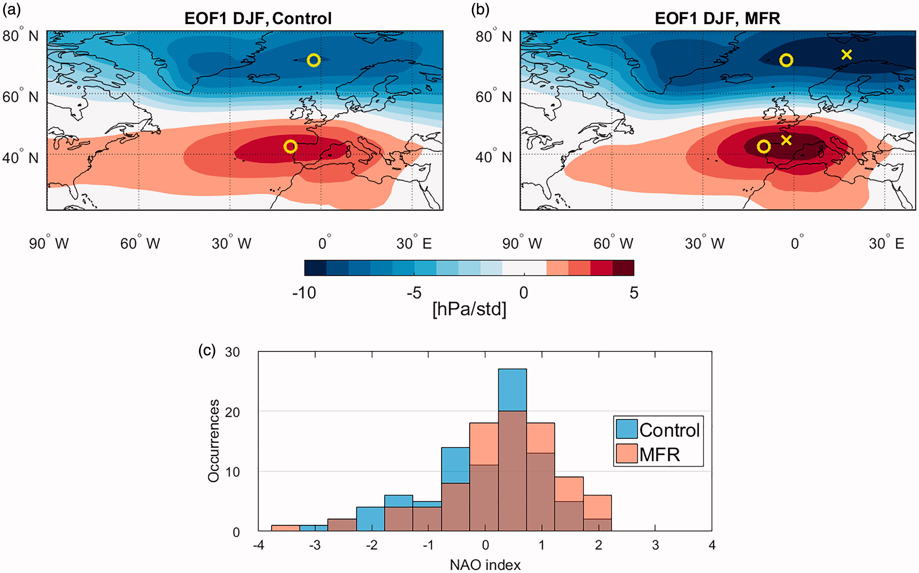
Fig. 3.
First EOF of sea level pressure for (a) the Control and (b) the MFR simulations, respectively. Circle (cross) markers indicate the Control (MFR) NACs. (c) Frequency distribution of the monthly NAOI for the Control (blue) and MFR (orange) simulations.
Atmospheric blocking refers to a situation where the climatological westerly flow is obstructed by a quasi-stationary area of high pressure. We identify blocks using the bi-dimensional instantaneous blocking (IB) index of Davini et al., (2012a). The algorithm is an extension of the one-dimensional Tibaldi and Molteni (1990) blocking index and is based on the reversal of the meridional gradient of 500 hPa geopotential height (Z500). The resulting IB index provides a binary time series for every grid point, indicating blocking activity. Details of how the index is calculated are provided in Text S4 in the Supplementary Material. Three regional blocking indices are defined as the average fraction of blocked days in the three domains marked by the black boxes in Fig. 4a. The three indices are referred to as Low, Mid and High-Latitude Blocking (LLB, MLB and HLB), respectively. The LLB region is intentionally located to the north-east of the subtropical blocking maximum, in order to capture the events having the greatest impact on the large-scale atmospheric flow over the European continent. The MLB index is positioned over the region where increased blocking is found in the MFR simulation. Finally, the HLB index is associated with Greenland blocking.
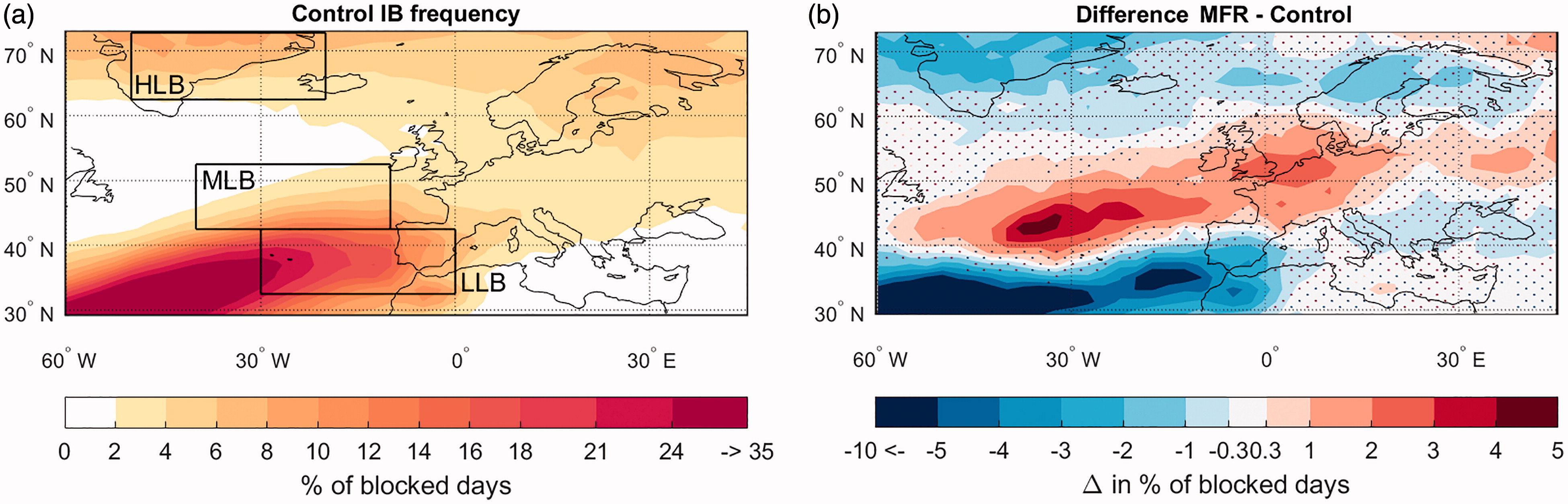
Fig. 4.
(a) Climatological DJF blocking frequency (% of blocked days) for the Control simulation. (b) changes in blocking frequency for the MFR scenario relative to the Control simulation. Stippling denotes areas where the difference is not significant at the 95% confidence level under a 2-sample t-test. The boxes in (a) mark the domains used to compute the low-, mid- and high-latitude blocking indices.
The latitude and speed of the eddy-driven jet stream in the North Atlantic region are identified using the low-level daily mean zonal wind field, following the methodology of Woollings et al. (2010). This method provides the zonal-averaged location of the jet latitude and corresponding average speed. Details of how the index is calculated are provided in Text S5 in the Supplementary Material.
We also discuss the skewness of probability distribution functions (PDFs), namely the distributions’ third standardised moment. A positive skewness indicates a greater weight of the right-hand tail of the distribution relative to the left-hand tail, thus indicating more frequent or larger positive deviations from the mean. The inverse is true for a negative skewness. As a caveat, we note that skewness alone does not distinguish between a fat, short tail and a long, thin tail, even though the difference between the two can be important in the context of PM2.5 threshold exceedances. Finally, we note that all significance tests are provided at the 5% significance level unless otherwise noted.
Results
3.
As first step, changes are investigated in the large-scale atmospheric circulation under MFR relative to the control simulation (Section 3.1). Then the impact of the changes on urban PM2.5 concentrations over Europe (Section 3.2) and the implications in terms of exceedances of air quality regulation thresholds are studied (Section 3.3).
Future atmospheric circulation changes
3.1.
The most evident large-scale change in the atmospheric circulation under the MFR scenario is a change in the spatial structure of the NAO. The maximum and minimum of the EOF – hereafter referred to as NAO centres (NACs) – display a substantial eastward shift (Figs. 3a,b). The northern NAC is displaced 20° eastward and 2° northward, while the southern NAC is displaced 7.5° eastward and 2° northward, moving further inland over the Iberian Peninsula. Furthermore, strengthening of both the northern and southern centres of action is seen, matching an increase in explained variance from 43% to almost 48%. The distribution of NAOI occurrences for the two simulations is shown in Fig. 3c. The MFR simulation shows a small but significant shift in the NAO mean state of +0.32 compared to the control simulation, combined with a more negatively skewed distribution (from −0.66 to −0.93). The shift in the mean dominates over the decrease in skewness, resulting in a large increase in strong positive NAO episodes 1 , from around 17% of the time in the control run to over 27% in the MFR scenario.
The shift in the NAO is indicative of a number of important changes in the atmospheric dynamics of the Euro-Atlantic sector, such as blocking episodes. The control simulation displays blocking maxima over the subtropics and Greenland, and a weaker blocking frequency over Europe (Fig. 4a). This spatial pattern is in reasonable agreement with the reanalysis data, although the model tends to overestimate subtropical blocking and underestimate high-latitude blocking and blocking over Europe (see Fig. S4). Similar biases in blocking frequency are found in a number of CMIP5 models (Anstey et al., 2013), and must be taken into account when interpreting the results. The MFR simulation displays a significant decrease in both high-latitude and low-latitude blocking activity, with an increase over the mid-Atlantic and continental Europe (Fig. 4b). The decrease in high-latitude blocking is consistent with previous studies that found its frequency to be anti-correlated with the NAOI (Woollings et al., 2008a) and its decrease to be associated with an eastward shift of the NAO pattern (Davini et al., 2012b). On the contrary, the strong decrease in subtropical blocking is not typically associated with a more positive NAO (e.g. Santos et al., 2013). We surmise that the north-eastward shift of the southern NAC in the MFR case leads to a corresponding shift in the peak blocking region, as for example discussed in the context of historical variability by Yao and Luo (2015). The resulting tri-polar anomaly pattern differs from previous simulations based on another climate model, which showed a dipole blocking anomaly under an MFR scenario with no significant changes in subtropical blocking frequency (Pausata et al., 2015). This discrepancy may be ascribed to the significant differences in the climatological blocking distributions of climate models (Anstey et al., 2013) and the equally significant differences in the exact locations of the NACs (Davini and Cagnazzo, 2014).
To further investigate the large-scale context in which the blocking anomalies occur, we analyse the associated changes in the North Atlantic jet stream. The jet’s variability influences the weather and climate of a large part of Europe, and in general the jet relates more directly to storm track characteristics than variability patterns based on SLP or geopotential fields (Athanasiadis et al., 2010). Furthermore, the large scale circulation over the North Atlantic can be interpreted as an alternance between blocked and unblocked zonal flow states (Woollings et al., 2008b), making the study of the jet’s variability a natural complement to that of changes in blocking frequencies. In reanalysis data, the PDF of jet latitude is tri-modal (Fig. S5; Woollings et al., 2010). Like most CMIP5 models, NorESM fails to reproduce this tri-modal distribution and only captures two modes, corresponding to the reanalysis distribution’s central and northern peaks (cf. Fig. 5a with Fig. S5a; see also Fig. 5 in Iqbal et al., 2017). This means that the jet stream in our model appears more often in the mid- and high-latitudes, which is consistent with the model’s blocking biases discussed above.
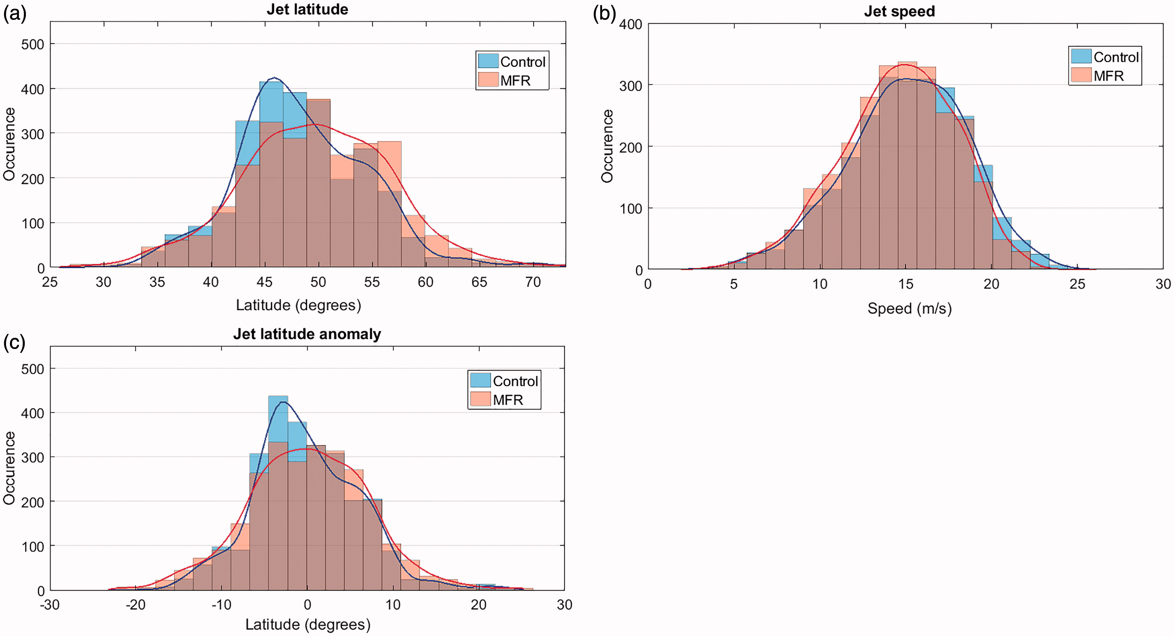
Fig. 5.
Frequency distributions of the daily DJF (a) jet latitude and (b) jet speed indices, for the Control (blue) and MFR (orange) simulations. Note that these are deviations from the seasonal cycle with the winter climatological means added back. (c) Displays the same distributions as (a) without the means added. The continuous curves are kernel estimations of the PDFs.
The MFR scenario shows a significant northward shift in the winter mean jet latitude by 1.34°, accompanied by a notable decrease in skewness (Fig. 5a). Woollings et al. (2011); Woollings and Blackburn (2012), among others, have shown that a northward displacement of the jet stream and storm track is expected under anthropogenic climate change. The preferred mid-latitude state of the jet (at around 45° N) is no longer apparent in the MFR simulation. Instead, a broad singular mode emerges over a band from roughly 42° up to 58° N, with a peak around 50° N. This results in a ∼5° northward shift in the mode of the distribution. Furthermore, the tails of the distribution become fatter, indicating more frequent extreme jet latitude occurrences on either side of its climatological location. This is evident when the two distributions are both centred at their respective means (Fig. 5c). There is also an increase in the variability of the jet position, with the standard deviation increasing from ∼6.1° to over 7°. These changes are consistent with the changes in blocking frequency seen in the MFR scenario: the increased mid-latitude blocking and decreased high-latitude and subtropical blocking favour northwards and southwards excursions of the jet, leading to a broader distribution and increased variability. The preference for an overall northward shift is due to the fact that subtropical blocking occurs with a much higher absolute frequency than high-latitude blocking in the MFR scenario (not shown), notwithstanding the large decrease in blocking frequency below ∼40° N relative to the control simulation (Fig. 4b). In addition to the changes in latitude, a significant decrease in the mean jet speed by 0.37 ms−1 is also found, again consistent with more frequent mid-latitude blocking (Fig. 5b).
Fig. 6 shows the regression patterns for blocking frequency (blocked days per month) on the jet latitude and jet speed indices in the control and MFR simulations. As expected, an increase in jet latitude is accompanied by a positive anomaly in mid-latitude blocking and a decrease in high-latitude blocking. The low latitude blocking, on the contrary, is most sensitive to changes in the jet speed, and the anomalies associated with a decreased jet speed closely match those seen for the MFR case relative to the control simulation (cf. Fig. 6d with Fig. 4b, keeping in mind that the sign of the former figure must be inverted to visualise the changes in blocking corresponding to a decrease in jet speed). However, the MFR jet speed decrease is insufficient to fully account for the negative anomaly in low-latitude blocking frequency. We therefore hypothesise that at least part of the anomalous decrease in low-latitude blocking could be due to the above-mentioned shift of the southern NAC.
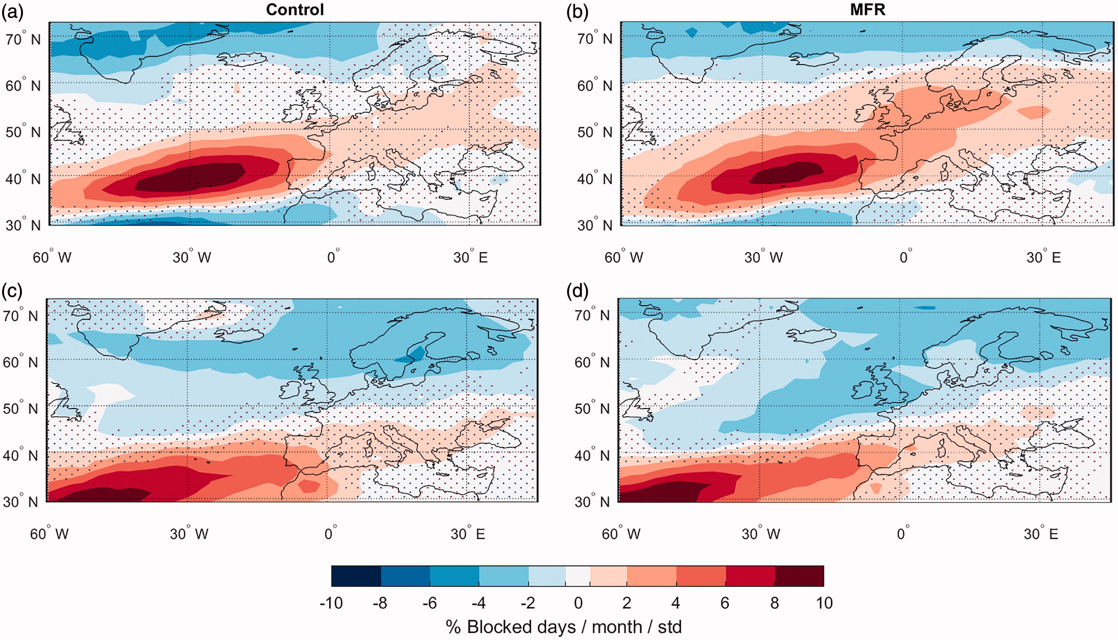
Fig. 6.
Regression patterns (% of blocked days/month/standard deviation) of blocking frequency on (a, b) jet latitude and (c, d) jet speed time series for the Control (a, c) and MFR (b, d) simulations during DJF. Stippling denotes areas where the regression is not statistically significant at the 95% confidence level, based on the standard error of the regression.
We conclude that the MFR scenario leads to a number of interlinked changes in the large-scale circulation, affecting both the NAO and blocking regimes, mirrored by significant changes in the North Atlantic Jet.
Impacts on urban PM2.5 concentrations
3.2.
The extent to which urban PM concentrations in Europe are influenced by the atmospheric circulation changes discussed above is assessed using linear regression analysis. This method is applied to every grid point, producing a regression map that gives the average change in PM2.5 for a one standard deviation (σ) change in the reference time series. The analysis is performed on the population-scaled urban centre PM2.5 anomalies, as described in Section 2.2. To obtain a complete overview of the circulation-induced PM2.5 changes, we use six reference atmospheric time series: the NAOI, the jet latitude and speed indices and three blocking indices (Low, Mid and High-Latitude Blocking, see Section 2.4). The regressions are presented for the combined predominantly anthropogenic aerosol components (BC, OM, SO4). These three species all have similar physical properties with regard to their size distributions and their individual regression patterns are very similar in shape (not shown), warranting the analysis of composite PM2.5 regressions.
The regression coefficients of anthropogenic aerosol concentrations with the NAOI display a strong dipole pattern, with decreased PM concentrations of more than 3 µg/m3/σ in Continental and Northern Europe and increased concentrations in excess of 1 µg/m3/σ in the Mediterranean region (Fig. 7a, colours). Especially over Continental and Northern Europe, these values correspond to very significant anomalies relative to the wintertime seasonal mean, with local deviations from the climatology in excess of 20% (Fig. 7a, contours). A similar pattern is seen in the MFR scenario (Fig. 7b), albeit with lower absolute values over Continental and Northern Europe and similar, if not locally stronger, changes over the Mediterranean (e.g. over Southern France) and parts of Western Russia. The eastward shift of the largest regression values is consistent with the large shift in the northern NAC (Fig. 3b), and is also mirrored in the regression pattern of the number of rainy days on the NAOI (Fig. S6). The strong decrease in anthropogenic aerosol emissions in the MFR simulation should naturally lead to a decrease in the absolute values of the regression coefficients. The picture seen in the Mediterranean and Western Russia, with similar or even larger absolute values associated with a large increase in fractional changes (Fig. 7b, contours), points to the importance of the large-scale circulation associated with the NAO in controlling future PM concentrations over these regions.
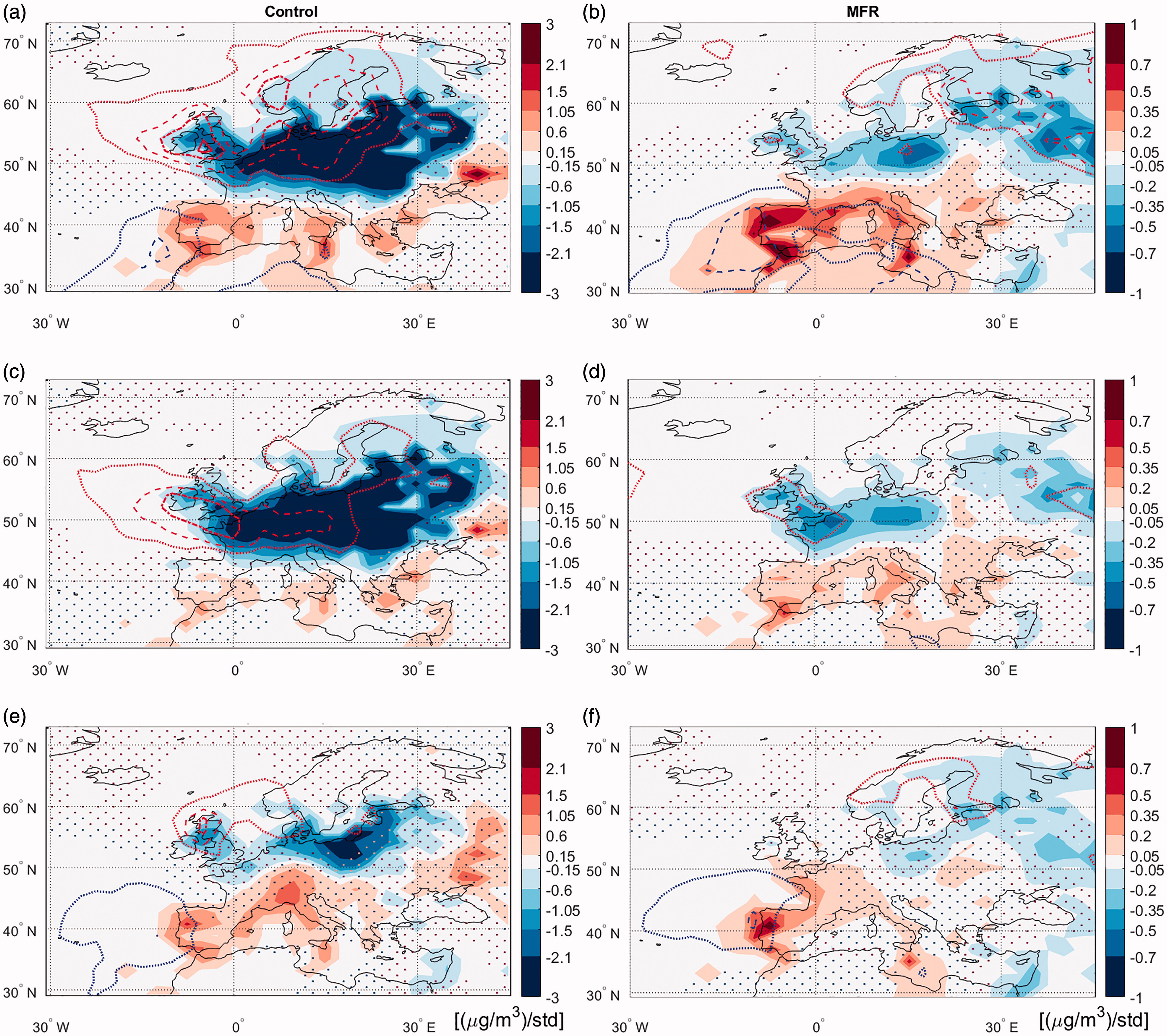
Fig. 7.
Regression patterns (µg/m3/standard deviation) of population-scaled urban anthropogenic PM2.5 anomalies on (a, b) the NAOI, (c, d) jet speed and (e, f) jet latitude indices, for the (a, c, e) Control and (b, d, f) MFR simulations during DJF. Line contours display positive (blue) and negative (red) departures from the DJF climatological mean, with contour intervals of 5%, starting from 10%. For enhanced visibility, contours change line style as follows: dotted, dashed, dash-dot, solid. Stippling denotes areas where the regression is not significant at the 95% confidence level, based on the standard error of the regression. Note that the colour scale ranges in the left and right-hand columns differ.
The regression coefficients of the two jet stream indices also yield dipolar patterns with negative regression values over Continental and Northern Europe and positive values over the Mediterranean region (Figs. 7c–f). However, negative regression values dominate the jet speed regression, especially in the control scenario. This suggests a very direct link to wet deposition removal rates. Consistently, we note that a faster jet is typically associated with a positive NAO and enhanced storminess over continental Europe (e.g. Woollings et al., 2008a; Messori and Caballero, 2015). The dipole regression associated with jet latitude displays a marked north-west to south-east tilt in the MFR simulation, with strong positive values over Northern Iberia and Western France and negative values mostly confined to Eastern Europe (Fig. 7f). At the same time, the regression of blocking on jet latitude in the MFR shows a broad region of positive values extending across the British Isles, France, and east to Denmark (Fig. 6b). This suggests that in the MFR scenario blocking can deflect the jet around this region when in its northern mode, limiting the associated PM2.5 concentration reductions.
The equivalent regression results for LLB, MLB and HLB indices are shown in Fig. 8. LLB is associated with a pattern similar to that seen for the jet latitude index. This can be explained by the fact that LLB leads to stagnating conditions over the Western Mediterranean, and shifts the jet stream to the north of its climatological location. MLB shows again a north-south dipole in the control simulation, but the dipole switches sign in the MFR case, displaying significant negative values over the central and western Mediterranean (cf. Figs. 8c, d). We surmise that this is linked to the jet speed. In the control simulation, MLB has a statistically significant correlation with jet latitude (0.60) but a weak correlation with jet speed (−0.14). This suggests that the jet shifts preferentially to the North when there is MLB and its speed is only marginally affected. In the MFR scenario, the correlation with jet latitude slightly weakens (0.55) while the correlation with jet speed becomes significant (−0.30). This points to an increased sensitivity of the jet speed to MLB, perhaps because the jet’s mean location in the MFR simulation is almost exactly at the centre of the MLB box. The weaker preference for a northward shift in the presence of MLB is consistent with the increased number of below-average jet latitude episodes shown in Fig. 5c. These two factors combined likely explain the negative regression values over the Mediterranean, in agreement with the patterns seen in Figs. 7d, f (note that the sign needs to be inverted to visualise the changes in PM2.5 concentrations corresponding to a decrease in jet latitude and speed). Finally, the HLB index shows a dipole with positive regression values over Continental Europe and negative values over the Mediterranean in both simulations. This pattern is fully consistent with the fact that, as discussed in Section 3.1, HLB is anti-correlated with the NAOI. All three blocking regressions are relatively weak because the strongest correlations are found at the locations of the blocking itself, namely over the North Sea and North Atlantic Ocean, where anthropogenic aerosols have low concentrations.
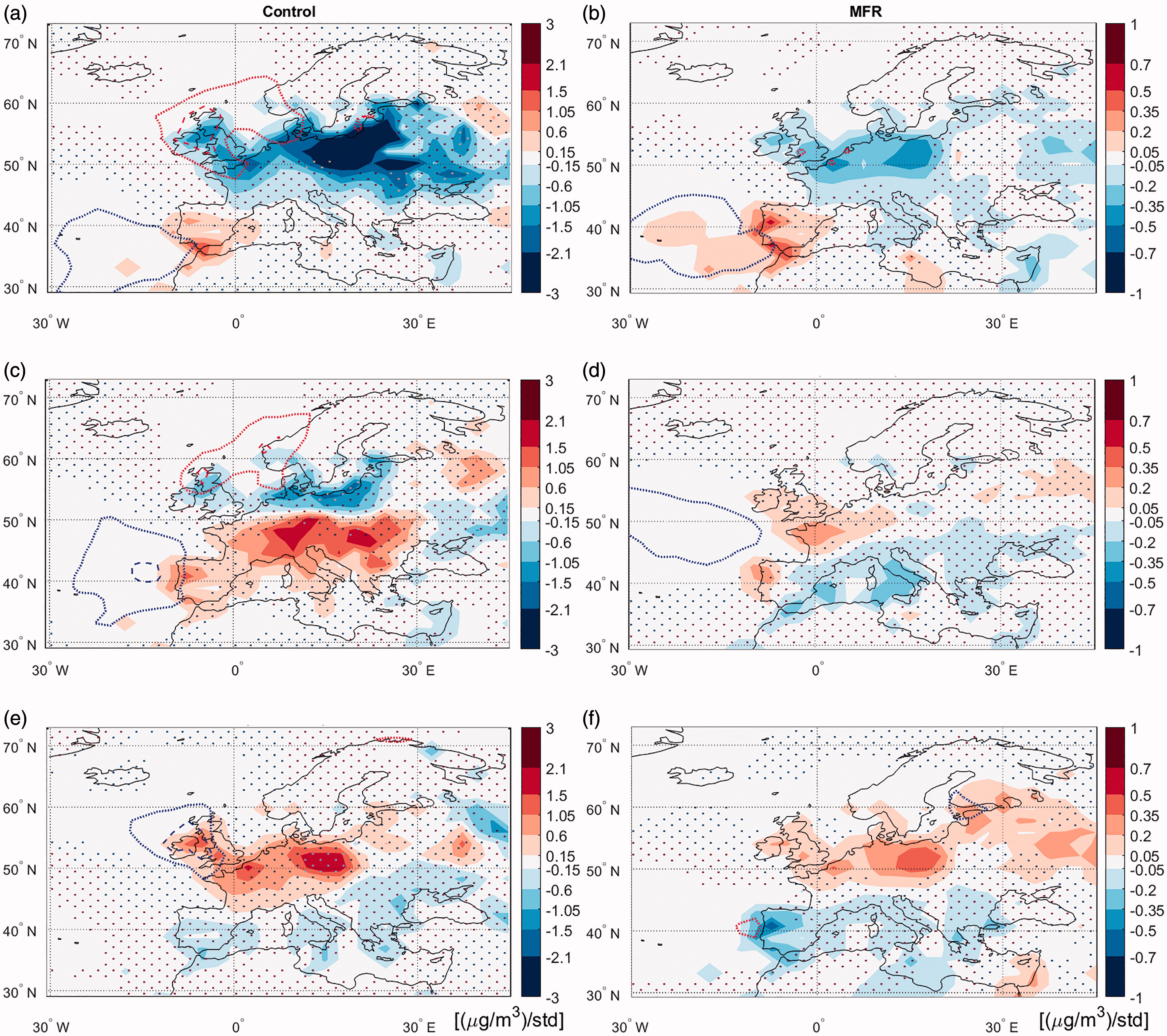
Fig. 8.
Regression patterns (µg/m3/standard deviation) of population-scaled urban anthropogenic PM2.5 anomalies on (a, b) LLB, (c, d) MLB and (e, f) HLB indices, for the (a, c, e) Control and (b, d, f) MFR simulations during DJF. Note that the colour scale ranges in the left and right-hand columns differ. All markings and colours are as in Fig. 7.
Regressions of the rainy day anomalies (% of rainy days per month) on the six atmospheric circulation indices discussed above closely resemble the anthropogenic PM2.5 regression patterns (see Fig. S6 for the NAOI, other indices not shown). Negative regressed rainy day values coincide with positive PM2.5 regressed values and vice versa. This suggests that, as hypothesised in our interpretation of the PM regressions, wet deposition is the main driver affecting the anthropogenic PM concentrations, in agreement with previous studies (Pausata et al. 2013, 2015). BC, OM and SO4 aerosol mass in the model used here mostly resides in small-size (Aitken and accumulation) modes, which makes the particles more sensitive to wet deposition via in-cloud or below-cloud scavenging, and less sensitive to dry deposition.
The overall impact of the changes in the above circulation features on the population-scaled urban centre PM2.5 concentrations can be summarised by weighting the regression values by the normalised change of the relevant circulation index and summing them. We term this quantity the climate penalty. The fractional and absolute climate penalties for both simulations are shown in Fig. 9. In the control scenario, the climate penalty closely matches the dipole regression pattern discussed above, with the atmospheric circulation leading to higher PM2.5 concentrations in the Mediterranean region and lower values in the Northern half of the continent (cf. Figs. 7, 8 and 9a, c). Calculating a climate penalty for the Control simulation tests the impact the MFR circulation changes would have if they were to occur under present-day PM concentrations. Part of the observed circulation changes are due to GHG forcing, and Pausata et al. (2015) have shown that the GHG-induced changes are similar in spatial pattern to those caused by a decrease in aerosols. The Control simulation climate penalty therefore paints a rough picture of a future world where no PM reduction measures have been put in place. For a more detailed analysis, beyond the scope of the present study, an ad-hoc simulation with increasing GHGs but fixed present-day aerosols would need to be performed. In the MFR, the climate penalty dipole becomes more zonally oriented, with lowered concentrations in Northern and Eastern Europe and heightened values in the Mediterranean and Western Europe (Fig. 9b, d), again closely resembling most of the regression patterns discussed previously. The relative anomalies associated with these changes are generally 5–15% in the control simulation and 2.5–15% in the MFR scenario.
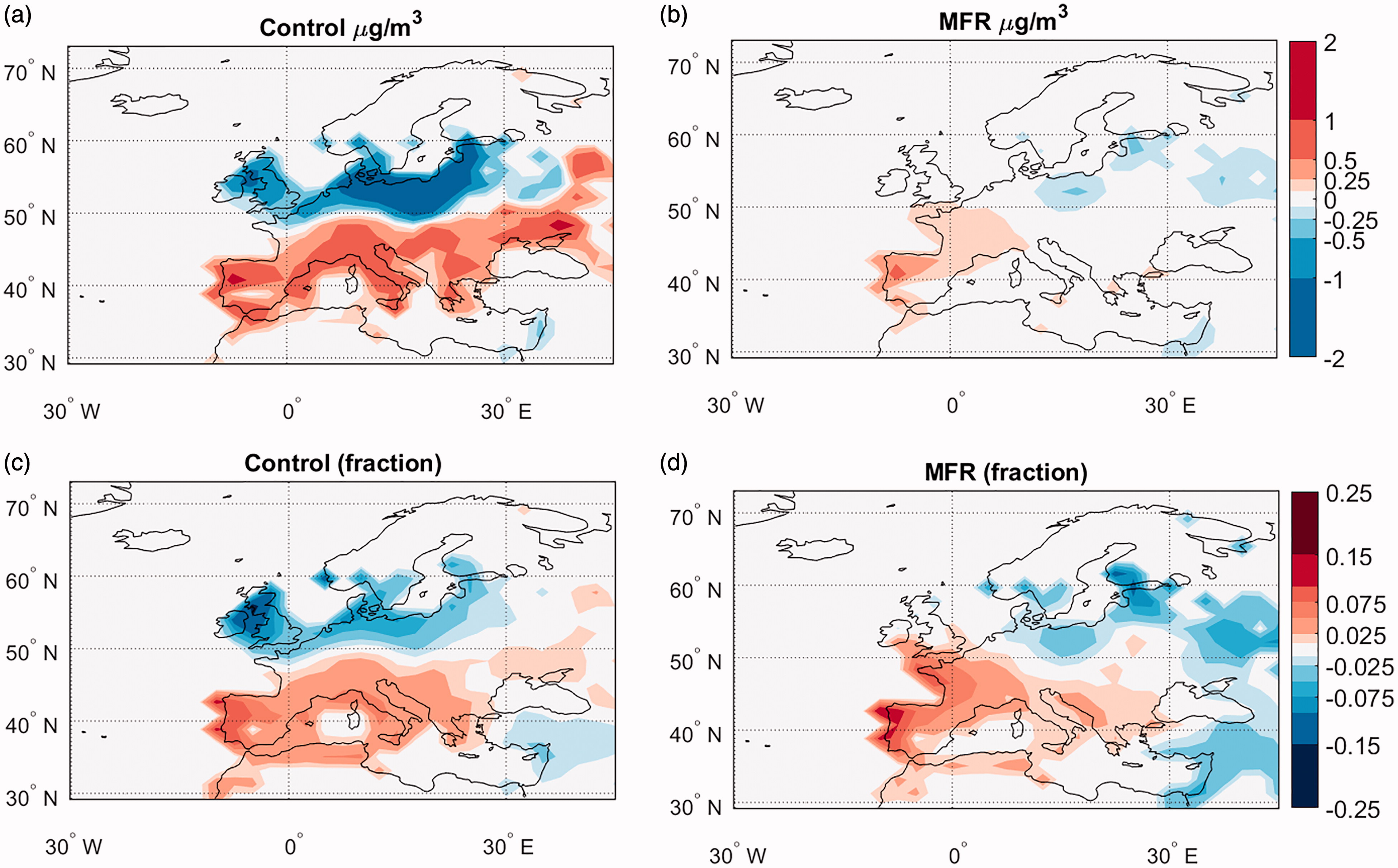
Fig. 9.
Climate penalty in PM2.5 concentrations for (a, c) the control and (b, d) the MFR simulations during DJF. This is expressed in terms of (a, b) absolute concentration values and (c, d) fractional changes relative to the DJF climatology.
Implications for air quality regulations
3.3.
The impact of large-scale circulation changes on PM concentrations is not limited to the climatological averages discussed in Section 3.2, but also leads to changes in severe PM pollution events. To quantify this latter aspect, we analyse the changes in the skewness of the anthropogenic PM2.5 concentration anomaly distributions between the two simulations (Fig. 10). The MFR results in a strong dipole, with negative values over Continental and Northern Europe and positive values over the Mediterranean region, largely mirroring the regression patterns shown in Fig. 7. This implies that positive urban PM2.5 daily concentration anomalies, relative to the baselines of the respective simulations, become more likely (or larger) in the Mediterranean and less likely (or smaller) in North-Western Europe under the MFR scenario.
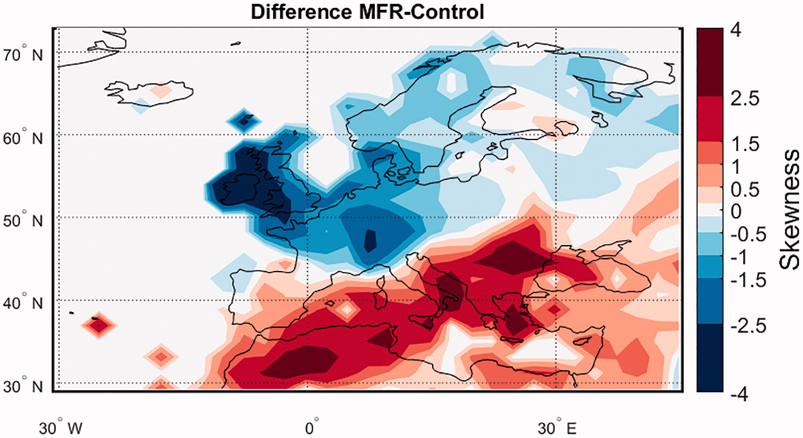
Fig. 10.
Difference in the skewness of the population-scaled urban anthropogenic PM2.5 between the Control and MFR simulations during DJF.
While a similar result had been previously reported by Pausata et al. (2015), an analysis of impacts on exceedances of regulatory thresholds was not carried out in that study. The population scaling we perform here allows us instead to address this point. The assessment is performed for urban centres, where exceedances mostly occur, and uses total urban PM2.5 concentrations (population scaled anthropogenic components + unscaled natural components) over the whole year. We consider two sets of PM2.5 concentration limits defined by the WHO: i) the IT-1 target annual (somewhat higher than the current EU legislation) and daily limits and ii) the AQG annual (significantly lower than the current EU legislation) and daily limits (see Section 2.3 and Table 4).
Exceedances of the daily and yearly IT-1 targets are mainly concentrated in Central-Eastern Europe, with peaks of 100 days/year and 30 out of 30 years of the simulation showing exceedances (Figs. 11a, c). If the more ambitious AQG limits are considered, extremely high exceedance rates are found across the continent. Much of Eastern Europe exceeds the daily AQG value on all days of the year, and virtually the whole of Europe exceeds the annual values on all 30 years of the simulation (Fig. 11b, d). This suggests that in the most polluted regions of Europe, PM2.5 concentrations routinely reach levels that can significantly impact public health. Moreover, most of the continent displays values which are above the ‘safe’ limits for human health indicated by the WHO (see Section 2.3).
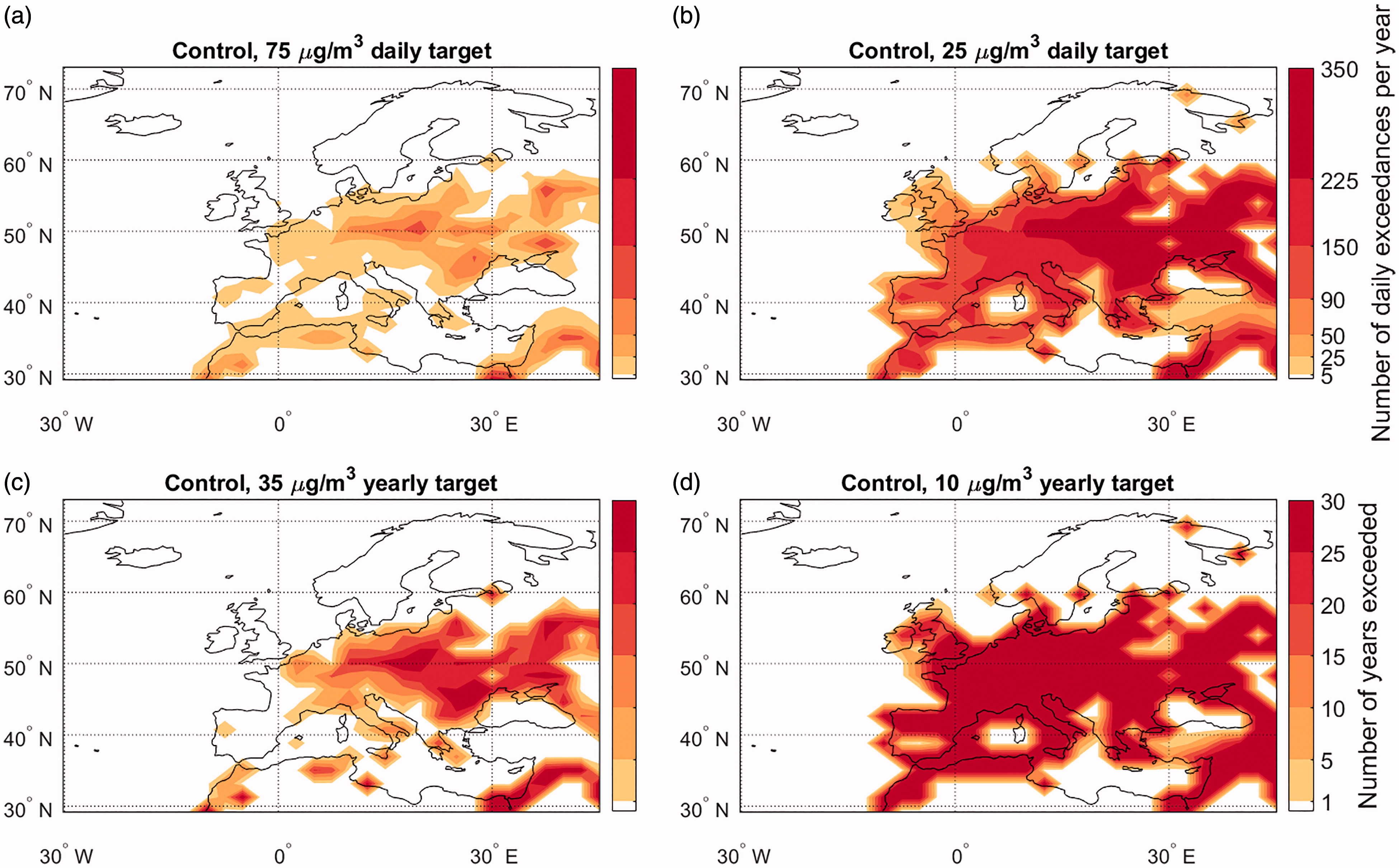
Fig. 11.
Exceedances of (a, c) the IT-1 and (b, d) the AQG PM2.5 aerosol limits in the control simulation. Results are expressed in terms of (a, b) the average number of days per year in which the daily targets were exceeded and (c, d) the number of years in which the yearly average targets were exceeded.
In the MFR scenario, the IT-1 annual target is never exceeded and the daily target is never exceeded for more than 5 days a year in any urban area in Europe (Figs. 12a, c). Below 40° N, dust intrusions from the Sahara lead to some exceedances. However, we note that the representation of dust in our simulations is highly simplified and subject to significant uncertainty. An MFR scenario would therefore be compatible with the IT-1 levels across the continent, even though we note that it is unlikely for these limits to remain unchanged in the coming decades. Under MFR, many cities in Northern Europe also meet the daily and annual AQG limits, while most areas in the Mediterranean and Central/Eastern Europe display exceedances for 25–150 days every year and for more than 20 of the 30 years considered (Figs. 12b, d). A comparison of Fig. 11 with Fig. 12 shows a clear shift in the regions with the most exceedances. In the control case, Central-Eastern Europe is the region displaying the most severe PM2.5 pollution. Under MFR, the most frequent AQG exceedances are instead seen over Central Europe and the Mediterranean. Over the latter regions, PM2.5 concentrations therefore remain above safe levels for human health even assuming a maximum feasible reduction scenario. For the current pollutant regulations (e.g. PM10), the EU allows a certain number of exceedances of the daily limits every year, while no exceedances are permitted for the yearly limits. A back-of-the-envelope calculation suggests that, fixing the variability in PM2.5 concentrations at MFR levels, the mean concentrations would need to drop by an additional 5 µg/m3 beyond the maximum feasible reduction in order to virtually eliminate (<1% of years and gridpoints) exceedances of the AQG yearly limit over Central and Southern Europe.
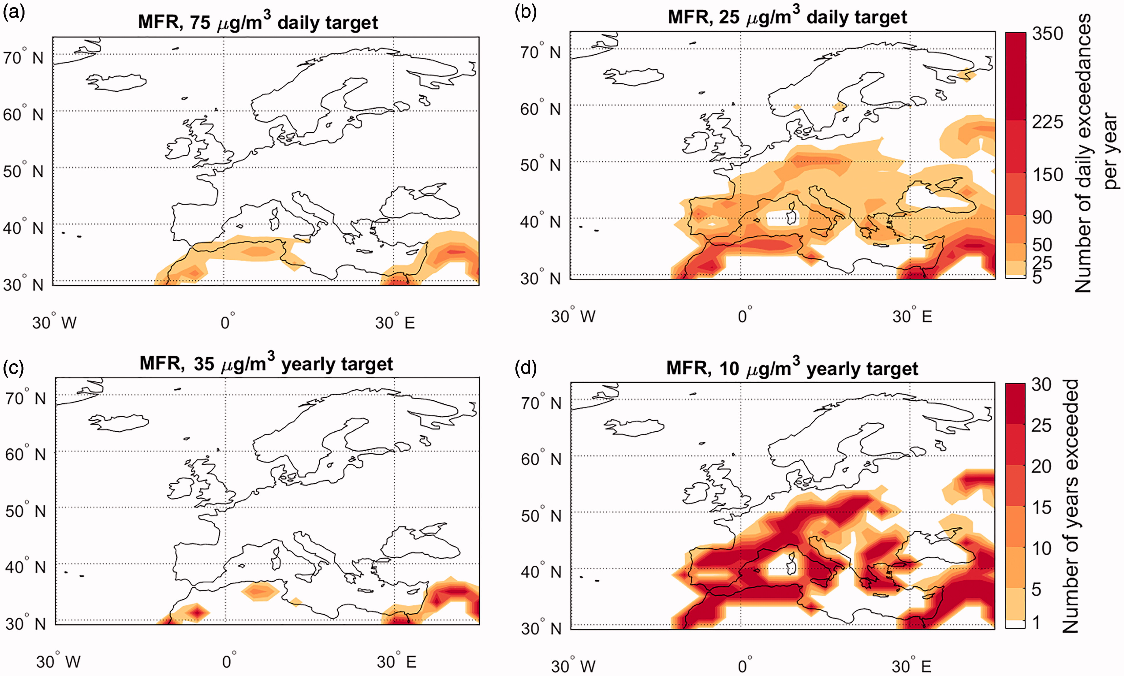
Fig. 12.
Exceedances of (a, c) the IT-1 and (b, d) the AQG PM2.5 aerosol limits in the MFR simulation. Results are expressed in terms of (a, b) the average number of days per year in which the daily targets were exceeded and (c, d) the number of years in which the yearly average targets were exceeded.
Discussion and conclusions
4.
The present paper analyses a future climate scenario over the Euro-Atlantic sector in which a maximum feasible reduction in aerosol emissions is implemented and GHG emissions follow an intermediate pathway (RCP4.5). This MFR simulation shows a shift towards a more positive NAO phase, accompanied by a north-eastward shift of the NAO centres (NACs). The significant increase in mean NAOI value is consistent with previous climate change and MFR simulations (e.g. Karpechko, 2010; Gillet and Fyfe, 2013; Pausata et al., 2015), as is the eastward shift of the variability pattern (Hu and Wu, 2004; Kuzmina et al., 2005; Dong et al., 2011; Pausata et al., 2015) which has itself been linked to a more positive NAO (Peterson et al., 2003). Even though the differences in the location of the NACs across different climate models can be very large (Davini and Cagnazzo, 2014), the eastward shift of the two poles under anthropogenic climate change scenarios therefore appears to be a robust result. Indeed, such a behaviour had already been noted in the previous generation of climate models (Ulbrich and Christoph, 1999). Moreover, a trend towards a more positive, eastward-shifted NAO has been observed in recent decades, although there is some debate as to whether it should be primarily ascribed to natural or forced variability (cf. Jung et al., 2003; Kuzmina et al., 2005; Dong et al., 2011).
In the present study, we have not attempted to separate the effects of GHG and aerosol changes on climate and air quality. Using the same model adopted here, Acosta Navarro et al. (2017) have shown that reduced aerosol emissions can lead to widespread changes in the large-scale dynamics and thermodynamics of the climate system. In particular, the authors found that an MFR scenario would lead to significantly more warming and a larger northward shift in the intertropical convergence zone than a scenario with increasing GHGs but aerosol emissions fixed at 2005 levels. Using the ECHAM5-HAM model, Pausata et al. (2015) have further shown that, in an MFR scenario, the aerosol reduction is the primary driver of the geographical shift in the NAO pattern.
The NAO is closely linked to a number of large-scale features of the atmospheric circulation. The shift in the NAO therefore reflects important dynamical changes. The MFR scenario is associated with an increased frequency of mid-latitude blocking and decreased frequencies over the northern North Atlantic and the subtropics. The mid-latitude blocking anomaly also displaces the jet stream from its climatological location, leading to a broader jet latitude distribution and a slightly lower climatological jet speed. A regression of blocking frequency on the jet speed and jet latitude paints a coherent picture, showing that the tripolar blocking frequency anomaly pattern found in the MFR scenario is, to a large degree, mirrored by the changes in the two jet indicators. A more positive NAO is typically associated with a more intense jet (e.g. Woollings et al., 2010); the significant decrease in jet speed found in the MFR scenario might therefore seem counter-intuitive. We ascribe this decrease to both the previously mentioned blocking changes and the fact that the jet speed metric adopted here only considers the zonal flow. A more positive NAO typically leads to an increase in the climatological south-west to north-east tilt of the jet (e.g. Messori and Caballero, 2015), associated with a strengthening of its meridional component. This is indeed found to be the case here, with the MFR scenario displaying an increase in the meridional component of the jet across most of the North Atlantic basin (Fig. S7). A caveat of our results is therefore that a purely zonal jet speed index might underestimate the intensification of the jet under positive NAO conditions.
The changes in large-scale atmospheric circulation have an important impact on the concentrations of anthropogenic PM2.5 in European urban areas. The changes in the NAO, jet stream and to a lesser degree blocking, lead to a dipole anomaly in the aerosol concentrations, with higher values in the broad Mediterranean and Western Europe regions and lower values in Continental and Northern Europe. This can be associated with changes in precipitation and the associated wet deposition of atmospheric aerosols. A positive NAO typically leads to wetter mid to high latitudes and a stronger Azores anticyclone with drier, more stable conditions than usual over the Mediterranean region. Similarly, the more northern location of the jet stream and the decrease in HLB leads to stormier weather and increased precipitation and wet deposition in Continental and Northern Europe. These findings are consistent with previous studies that analysed the impact of the NAO on aerosol concentrations (Pausata et al., 2013) and the NAO and blocking changes associated with an MFR scenario (Pausata et al., 2015). The present work additionally shows that the changes in blocking and the NAO are accompanied by significant anomalies in the jet stream, which in turn play an important role in controlling the PM concentrations. Indeed, the additional indices considered here can have important regional impacts and are necessary to gain a more nuanced and dynamically complete picture of the large-scale circulation impact on the PM2.5 concentrations across the European continent. This study further provides a coherent and complete picture of both atmospheric changes in a future climate with increasing GHG concentrations and reduced aerosol emissions and their impact on urban aerosol concentrations: two elements which had previously been analysed separately.
The new urban downscaling which we adopt, allows to contextualise the simulated PM2.5 changes relative to initial and long-term target concentrations set by the World Health Organisation. The initial target is to keep the concentrations below levels which are known to lead to a significant increase in mortality (IT-1 limits). The longer-term aim is to bring the PM2.5 concentrations below levels which are known to be harmful to human health (AQG limits). The MFR scenario assumes the optimal implementation of the most advanced currently available technologies, resulting in some of the lowest total aerosol column burdens among a range of possible future scenarios (e.g. Acosta-Navarro et al., 2017). One might therefore hope that this scenario corresponds to PM2.5 concentrations below harmful levels. Our results show that this is only partially true. On the one hand, the MFR scenario leads to virtually no exceedances of IT-1 levels in Europe, and largely meets the AQG limits over the northern part of the continent. On the other hand, the Mediterranean and Central/Western Europe will see a high frequency of exceedances of AQG limits. This can be partially explained by the large-scale circulation changes simulated in the MFR scenario, which lead to both an increased PM variability and increased average concentrations over the latter regions. As discussed in Section 3.2 above, this climate penalty leads to relative increases in PM2.5 concentrations of the order of 10–15% over large parts of France and the Iberian Peninsula while driving a net benefit over parts of Continental and Northern Europe. We therefore conclude that urban areas in the Mediterranean region are likely to frequently experience harmful PM2.5 concentrations in the future, even under the assumption of a strong decrease in aerosol emissions. As a caveat, we note that the downscaling method applied here may introduce significant uncertainty in calculating the exceedances, which should be taken into account when interpreting the quantitative results discussed here. For further details the reader is referred to Text S2 in the Supplementary Material. We further note that, as the concentration of anthropogenic PM2.5 decreases, the relative importance of natural aerosols will increase. In fact, in regions such as the Iberian Peninsula present-day high PM concentrations are already often associated with PM of natural origin (Pey et al., 2013; AIRUSE, 2015; Liora et al., 2016). In a future world with lower anthropogenic aerosol emissions and more stringent regulations, atmospheric circulation changes will become crucial in affecting the exceedances via changes in the emission, transport and removal of natural aerosols. This poses a serious challenge for both the design of future EU regulations and the implementation of aerosol reduction measures. Future regulations and long-term aerosol emission scenarios need to balance the competing requests of setting targets which are realistic and account for the underlying challenges to climate change mitigation and adaptation (Rao et al., 2017) while at the same time protecting public health. Reduction measures need to be tailored to these targets but must also take into account the fact that shifts in the large-scale atmospheric circulation will have diverging regional effects and change the relative importance of natural versus anthropogenic aerosols. Both natural and anthropogenic aerosols impact human health (e.g. Pöschl, 2005), and indeed high natural aerosol concentrations can lead to significant increases in cardiovascular hospitalisations and mortality in Europe (e.g. Alessandrini et al., 2013; Goudie, 2014, and references therein). However, for a given exposure level anthropogenic aerosols are likely to have more severe effects than natural ones such as dust or sea-salt (e.g. Slama Lighty et al., 2000; Anenberg et al., 2012). This may mitigate the impacts of the high future PM concentration values simulated in the Mediterranean region. While beyond the scope of the present study, targeted simulations investigating the role of natural aerosols such as sea salt and dust emission from North Africa would therefore greatly advance our understanding of the topic.
More generally, our conclusions point to the need for a systematic investigation of the atmospheric circulation associated with a variety of future scenarios, using a range of climate models. Indeed, the differences between individual models can result in different conclusions concerning how the large-scale circulation and aerosol concentrations change and interact. As an example, we note the discrepancy between the present study and a previous work by Pausata et al. (2015), discussed in Section 3.1, concerning the changes in subtropical blocking under an MFR scenario. Further investigations using the same MFR experiment for the largest possible number of CMIP5 (or future CMIP6) models would provide a better understanding of the spread in results and a valuable indication of the most robust features in the response of PM2.5 concentrations to circulation changes. A complementary approach would be to focus on downscaling with regional climate models including a more complete chemistry, in order to better understand population exposure and feedbacks on emissions and removals of both anthropogenic and natural aerosols.
An additional aim for future studies would be a more detailed analysis of the size distribution of atmospheric aerosols (e.g. Stanier et al., 2004; Manigrasso, 2012). Indeed, bulk PM concentrations give an incomplete image of air pollution impacts on human health, since fine and ultra-fine (<1 µm) particles could be more dangerous than those included in the currently used PM classing (Pope and Dockery, 2006). Furthermore, the chemical composition and possible toxicity of the particles is not directly considered when focusing on PM. Efforts in this direction would benefit from recent station measurements of continuous size distributions, which present a major advance over the traditional PM measurements (e.g. Asmi, 2011).
Disclosure statement
No potential conflict of interest was reported by the authors.
Supplemental data
Supplemental data for this article can be accessed here.